Astrophysics
Overview unavailable.
Astrophysics Overview
- Table of contents for Stan Owocki’s Fundamentals of Astrophysics.
- Organized into five major parts: stellar properties, stellar structure and evolution, interstellar matter and planet formation, galaxies, and cosmology.
- Covers methods for inferring stellar distances, luminosities, temperatures, radii, masses, rotation, ages, and velocities.
- Introduces broader astrophysical topics including the Sun, star formation, exoplanets, the Milky Way, external galaxies, dark matter, and active galactic nuclei.
- Concludes with cosmology topics such as universal expansion, dark energy, the Big Bang, cosmic microwave background, nucleosynthesis, and inflation, plus appendices on atomic physics and radiative transfer.
Fundamentals of Astrophysics
Stan Owocki
Contents
Part I Stellar Properties page 1
1 Introduction 3
1.1 Observational vs. Physical Properties of Stars 3
1.2 Scales and Orders of Magnitude 5
1.3 Questions and Exercises 9
2 Inferring Astronomical Distances 10
2.1 Angular size 10
2.2 Trignonometric parallax 12
2.3 Determining the Astronomical Unit (au) 15
2.4 Solid angle 15
2.5 Questions and Exercises 16
3 Inferring Stellar Luminosity 18
3.1 \Standard Candle" methods for distance 18
3.2 Intensity or Surface Brightness 19
3.3 Apparent and absolute magnitude and the distance modulus 20
3.4 Questions and Exercises 21
4 Inferring Surface Temperature from a Star's Color and/or Spectrum 23
4.1 The wave nature of light 24
4.2 Light quanta and the Black-Body emission spectrum 24
4.3 Inverse-temperature dependence of wavelength for peak
ux 26
4.4 Inferring stellar temperatures from photometric colors 26
4.5 Questions and Exercises 27
5 Inferring Stellar Radius from Luminosity and Temperature 29
5.1 Stefan-Boltzmann law for surface
ux from a blackbody 29
5.2 Questions and Exercises 30
6 Absorption Lines in Stellar Spectra 31
6.1 Elemental composition of the Sun and stars 33
4 Contents
6.2 Stellar spectral type: ionization abundances as temperature
diagnostic 34
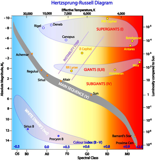
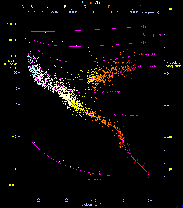
6.3 Hertzsprung-Russell (H-R) diagram 35
6.4 Questions and Exercises 36
7 Surface Gravity and Escape/Orbital Speed 37
7.1 Newton's law of gravitation and stellar surface gravity 37
7.2 Surface escape speed Vesc 38
7.3 Speed for circular orbit 39
7.4 Virial Theorum for bound orbits 39
7.5 Questions and Exercises 40
8 Stellar Ages and Lifetimes 42
8.1 Shortness of chemical burning timescale for Sun and stars 42
8.2 Kelvin-Helmholtz timescale for gravitational contraction 42
8.3 Nuclear burning timescale 43
8.4 Age of stellar clusters from main-sequence turno
point 44
8.5 Questions and Exercises 45
9 Inferring Stellar Space Velocities 47
9.1 Transverse speed from proper motion observations 47
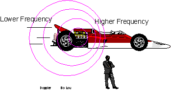
9.2 Radial velocity from Doppler shift 49
9.3 Questions and Exercises 50
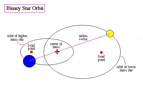
10 Using Binary Systems to Determine Masses and Radii 51
10.1 Visual binaries 51
10.2 Spectroscopic binaries 53
10.3 Eclipsing binaries 55
10.4 Mass-Luminosity scaling from astrometric and eclipsing binaries 56
10.5 Questions and Exercises 57
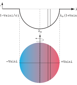
11 Inferring Stellar Rotation 59
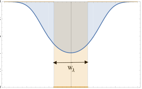
11.1 Rotational broadening of stellar spectral lines 59
11.2 Rotational period from starspot modulation of brightness 61
11.3 Questions and Exercises 62
12 Light Intensity and Absorption 63
12.1 Intensity vs. Flux 63
12.2 Absorption mean-free-path and optical depth 65
12.3 Inter-stellar extinction and reddening 67
12.4 Questions and Exercises 68
13 Observational Methods 69
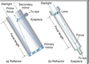
13.1 Telescopes as light buckets 69
Contents 5
13.2 Angular resolution 70
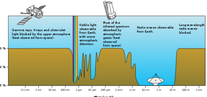
13.3 Space-based missions 72
13.4 Questions and Exercises 73
14 Our Sun 74
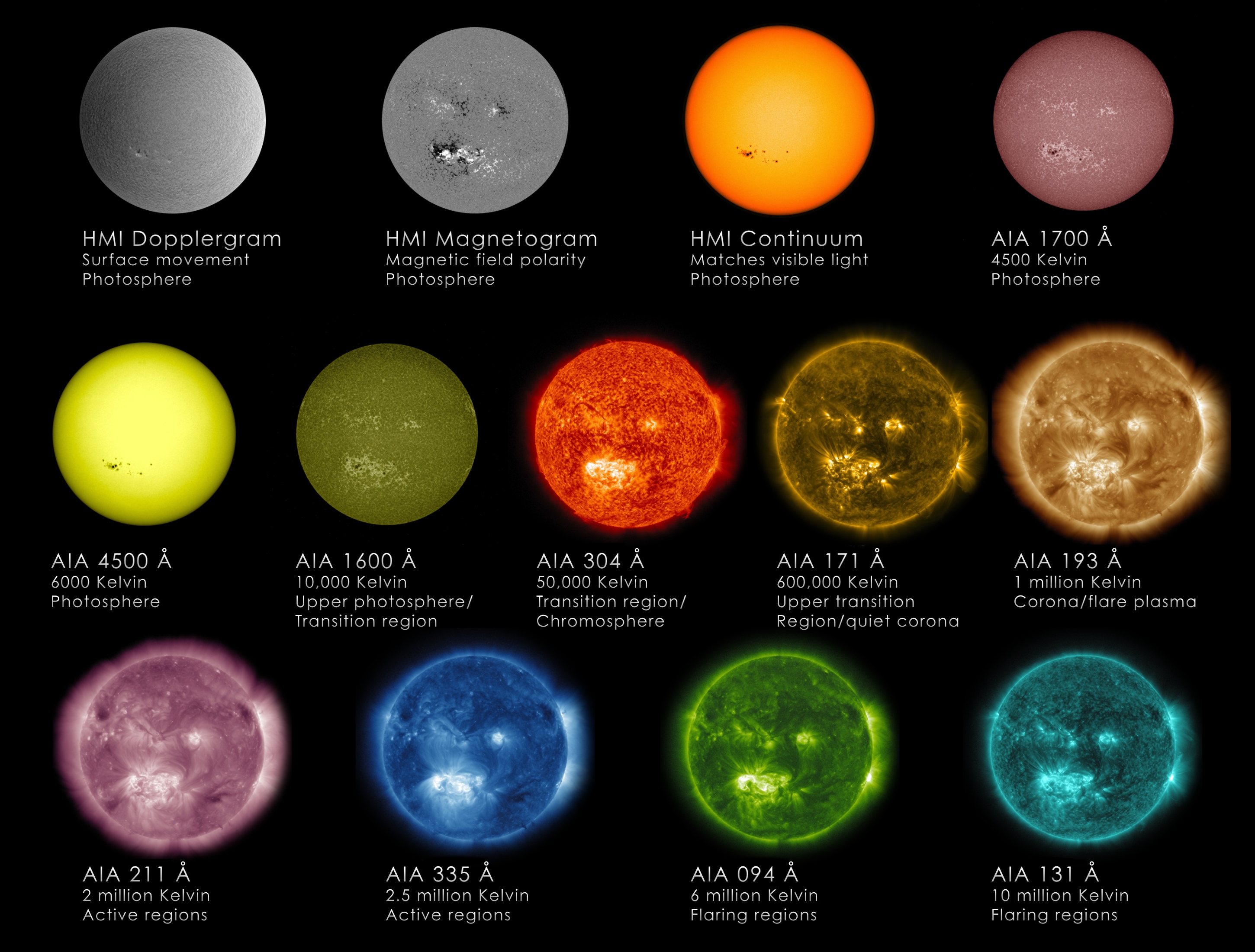
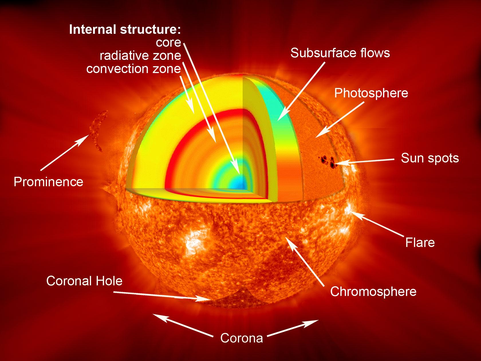
14.1 Imaging the solar disk 74
14.2 Corona and solar wind 76
14.3 Convection as a driver of solar structure and activity 78
14.4 Questions and Exercises 80
Part II Stellar Structure & Evolution 81
15 Hydrostatic Balance between Pressure and Gravity 83
15.1 Hydrostatic equilibrium 83
15.2 Pressure scale height and thinness of surface layer 85
15.3 Hydrostatic balance in stellar interior and the virial temperature 86
15.4 Questions and Exercises 87
16 Transport of Radiation from Interior to Surface 88
16.1 Random walk of photon di
usion from stellar core to surface 88
16.2 Di
usion approximation at depth 90
16.3 Atmospheric variation of temperature with optical depth 91
16.4 Questions and Exercises 91
17 Structure of Radiative vs. Convective Stellar Envelopes 92
17.1LM3relation for hydrostatic, radiative stellar envelopes 92
17.2 Horizontal-track Kelvin-Helmholtz contraction to the main sequence 93
17.3 Convective instability and energy transport 94
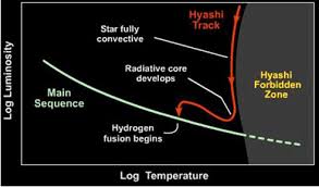
17.4 Fully convective stars { the Hayashi track for proto-stellar
contraction 96
18 Hydrogen Fusion and the Mass Range of Stars 98
18.1 Core temperature for H-fusion 99
18.2 Main sequence scalings for radius-mass and luminosity-temperature 100
18.3 Lower mass limit for hydrogen fusion: Brown Dwarf stars 101
18.4 Upper mass limit for stars: the Eddington Limit 102
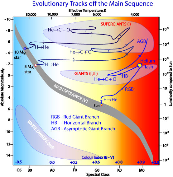
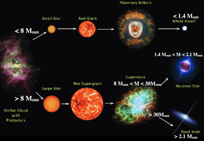
19 Post-Main-Sequence Evolution: Low-Mass Stars 104
19.1 Core-Hydrogen burning and evolution to the Red Giant branch 105
19.2 Helium
ash and core-Helium burning on the Horizontal Branch 106
19.3 Asymptotic Giant Branch to Planetary Nebula to White Dwarf 108
19.4 White Dwarf stars 108
19.5 Chandasekhar limit for white-dwarf mass: M < 1:4M
109
6 Contents
20 Post-Main-Sequence Evolution: High-Mass Stars 111
20.1 Multiple shell burning and horizontal loops in H-R diagram 111
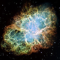
20.2 Core-collapse supernovae 112
20.3 Neutron stars 114
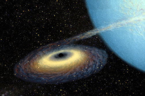
20.4 Black Holes 114
20.5 Observations of stellar remnants 116
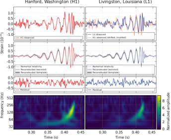
20.6 Gravitational Waves from Merging Black Holes or Neutron Stars 118
20.7 Questions and Exercises 121
Part III Interstellar Medium & Formation of Stars and Planets 123
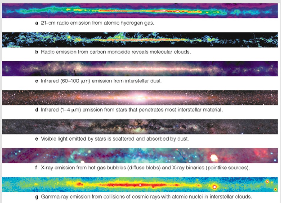
21 The Interstellar Medium 125
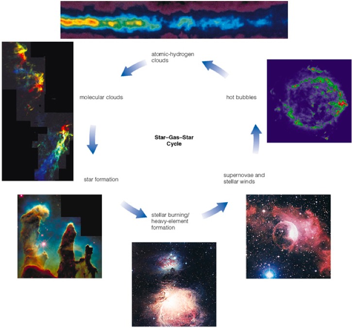
21.1 Star-gas cycle 125
21.2 Cold-Warm-Hot phases of nearly isobaric ISM 126
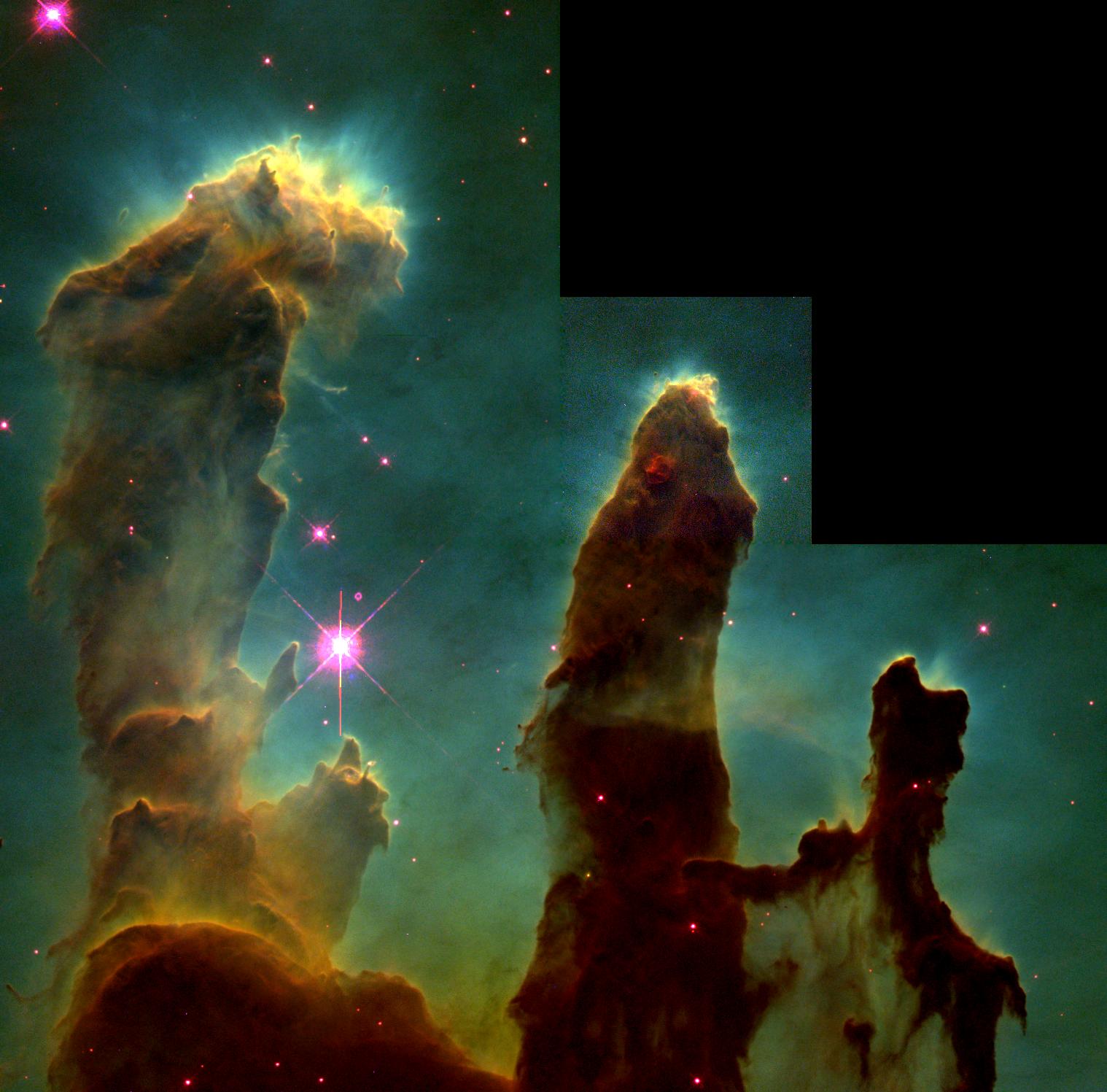
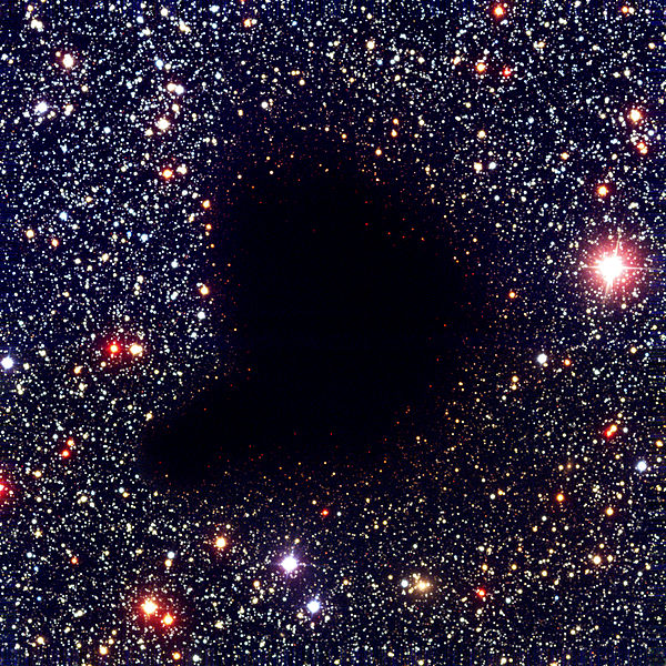
21.3 Molecules and dust in cold ISM: Giant Molecular Clouds 129
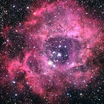
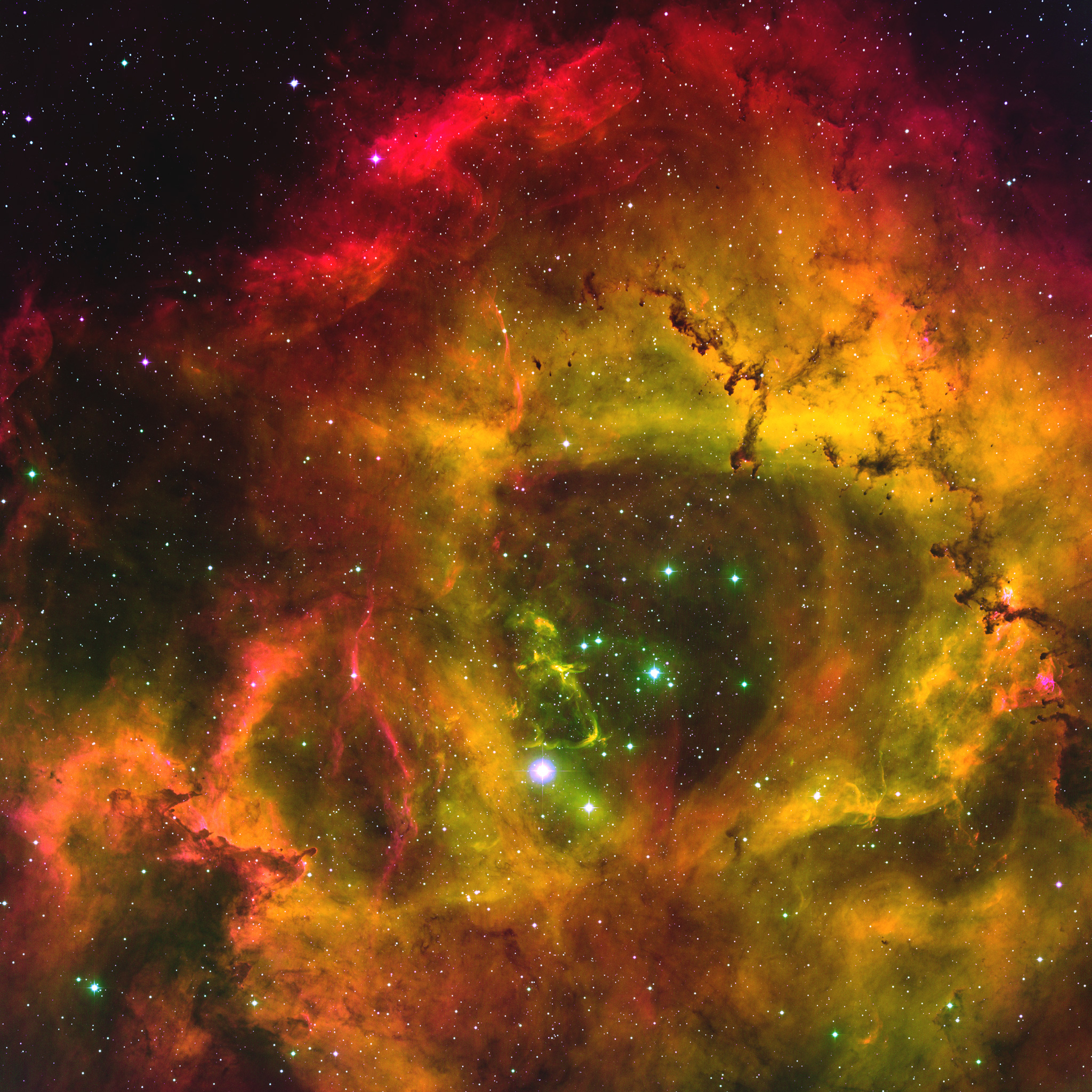
21.4 HII regions 132
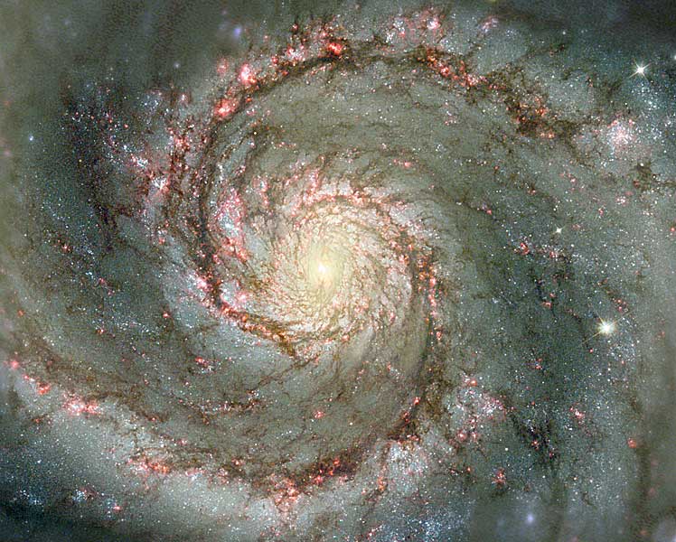
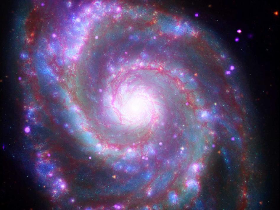
21.5 Galactic organization of ISM and star-gas interaction along spiral
arms 134
22 Star Formation 136
22.1 Jeans Criterion for gravitational contraction 136
22.2 Cooling by molecular emission 137
22.3 Free-fall timescale and the galactic star formation rate 138
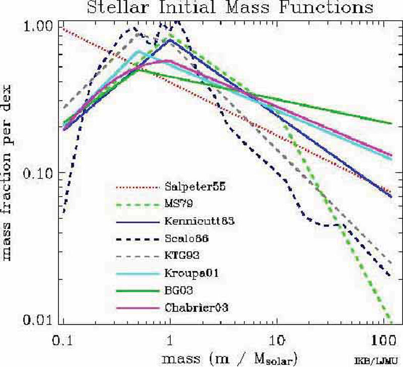
22.4 Fragmentation into cold cores and the Initial Mass Function (IMF) 139
22.5 Angular momentum conservation of rotating cores and disk
formation 140
22.6 Questions and Exercises 142
23 Origin of Planetary Systems 144
23.1 The Nebular Model 144
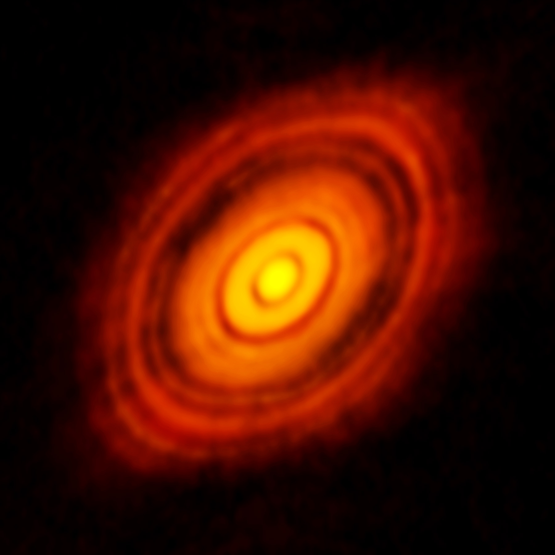
23.2 Observations of Protoplanetary Disks 145
23.3 Our Solar System 146
23.4 The Ice Line: Gas Giants vs. Rocky Dwarfs 147
23.5 Equilibrium Temperature 148
23.6 Questions and Exercises 148
24 Water Planet Earth 149
24.1 Formation of Moon by Giant Impact 149
24.2 Water from Icy Asteroids 150
24.3 Our Magnetic Shield 151
24.4 Life from Oceans: Earth vs. Icy Moons 151
24.5 Questions and Exercises 152
25 Extra-Solar Planets 153
Contents 7
25.1 Direct Imaging Method 153
25.2 Radial Velocity Method 154
25.3 Transit Method 155
25.4 The Exoplanet Census: 4000+ and counting 157
25.5 Search for Earth-sized Planets in the Habitable Zone 158
25.6 Questions and Exercises 159
Part IV Our Milky Way & Other Galaxies 161
26 Our Milky Way Galaxy 163
26.1 Disk, halo, and bulge components of the Milky Way 163
26.2 Virial mass for cluster from stellar velocity dispersion inferred
from Doppler shifts 166
26.3 Galactic rotation curve & dark matter 168
26.4 Super-massive black hole at the galactic center 171
27 External Galaxies 174
27.1 Cepheid variables as standard candle for distances to external
galaxies 174
27.2 Galactic redshift and Hubble's law for expansion 175
27.3 Tully-Fisher Relation: Lgal/V4
rot 177
27.4 Spiral, Elliptical, & Irregular galaxies 179
27.5 Role of Galaxy Collisions 181
28 Active Galactic Nuclei (AGNs) and Quasars 182
28.1 Basic properties and model 182
28.2 Lyman alpha clouds 183
28.3 Gravitational lensing of quasar light by foreground Galaxy Clusters 185
28.4 Gravitational redshift 187
28.5 Apparent \super-luminal" motion of quasar jets 187
29 Large Scale Structure and Eras in the Evolution of the Universe 191
29.1 Galaxy clusters & super-clusters 191
29.2 Dark matter: Hot vs. Cold, WIMPs vs. MACHOs 192
Part V Cosmology 195
30 Newtonian Dynamical Model of Universe Expansion 197
30.1 Critical Density 197
30.2 Gravitational deceleration of increasing scale factor 198
30.2.1 Critical Universe,
m= 1 200
30.2.2 Closed Universe,
m>1 200
30.2.3 Open Universe,
m<1 201
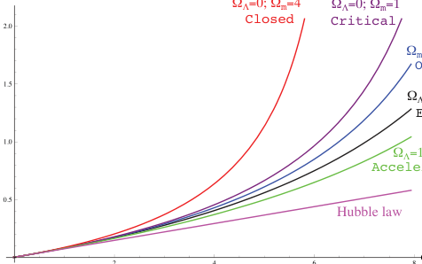
30.3 Redshift vs. distance: Hubble law for various expansion models 201
8 Contents
30.4 Questions and Exercises 203
31 Accelerating Universe with a Cosmological Constant 205
31.1 White-dwarf supernova as distant standard candles 205
31.2 Cosmological Constant and Dark Energy 206
31.3 Flat Universe with Dark Energy 208
31.3.1 Exponential expansion of
at, matter-empty universe 208
31.3.2 General solutions for
at universe with dark energy 208
31.4 The \Flatness" problem 209
32 The Hot Big Bang 211
32.1 The temperature history of the universe 211
32.2 Discovery of the Cosmic Microwave Background (CMB) 212
32.3 Fluctuation Maps from COBE, WMAP, Planck 213
33 Eras in the Evolution of the Universe 216
33.1 Matter-dominated vs. Radiation-dominated eras 216
33.2 The recombination era 217
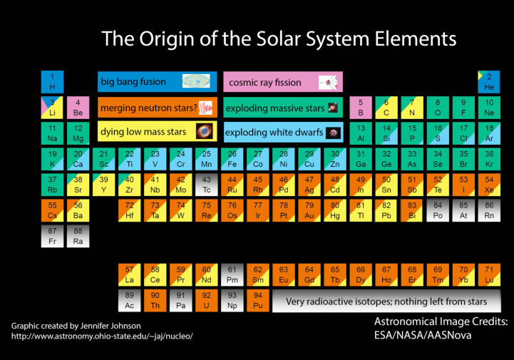
33.3 Era of nucleosynthesis 219
33.4 The particle era 220
33.5 Questions and Exercises 222
34 Cosmic in
ation 223
34.1 Problems for standard Hot Big Bang model 223
34.2 The era of cosmic in
ation 223
Appendix A Atomic Energy Levels and Transitions 226
Appendix B Equilibrium Excitation and Ionization Balance 231
Appendix C Atomic origins of opacity 234
Appendix D Radiative Transfer 238
Part I
Stellar Properties
1 Introduction
1.1 Observational vs. Physical Properties of Stars
Fundamental Properties of Stars
- Stars appear as points of light due to their immense distance, which prevents telescopes from resolving their physical surfaces like we do with the Sun.
- The Sun serves as a critical local benchmark, allowing astronomers to scale physical properties like mass and temperature to more distant stellar objects.
- Stellar positions are measured using celestial coordinates, with modern space telescopes achieving milli-arcsec precision by avoiding atmospheric distortion.
- Trigonometric parallax uses the Earth's orbital motion to calculate the distance to nearby stars based on shifts in their apparent position.
- Apparent brightness is quantified as energy flux, though the historical magnitude system remains in use due to the human eye's logarithmic response to light.
Of course, when we actually do so, the values we obtain dwarf anything we have direct experience with, thus stretching our imagination, and challenging the physical intuition and insights we instinctively draw upon to function in our own everyday world.
What are the key physical properties we can aspire to know about a star? When
we look up at the night sky, stars are just little \points of light", but if we look
carefully, we can tell that some appear brighter than others, and moreover that
some have distinctly di
erent hues or colors than others. Of course, in modern
times we now know that stars are really \Suns", with properties that are similar
{ within some spread { to our own Sun. They only appear much much dimmer
because they are much much further away. Indeed they appear as mere \points"
because they are so far away that ordinary telescopes almost never can actually
resolve a distinct visible surface, the way we can resolve, even with our naked
eye, that the Sun has a
nite angular size.
Because we can resolve the Sun's surface and see that it is nearly round, it is
perhaps not too hard to imagine that it is a real, physical object, albeit a very
special one, something we could, in principle \reach out and touch". (Indeed a
small amount of solar matter can even travel to the vicinity of the Earth through
the solar wind, coronal mass ejections, and energetic particles.) As such, we can
more readily imagine trying to assign values of common physical properties {
e.g. distance, size, temperature, mass, age, energy emission rate, etc. { that we
regularly use to characterize objects here on Earth. Of course, when we actually
do so, the values we obtain dwarf anything we have direct experience with, thus
stretching our imagination, and challenging the physical intuition and insights we
instinctively draw upon to function in our own everyday world. But once we learn
to grapple with these huge magnitudes for the Sun, we then have at our disposal
that example to provide context and a relative scale to characterize other stars.
And eventually as we move on to still larger scales involving stellar clusters or
even whole galaxies, which might contain thousands, millions, or indeed billions
of individual stars, we can try at each step to develop a relative characterization
of the scales involved in these same physical quantities of size, mass, distance,
etc.
So let's consider here the properties of stars, identifying
rst what we can
directly observe about a given star. Since, as we noted above, most stars are
e
ectively a \point" source without any (easily) detectable angular extent, we
might summarize what can be directly observed as three simple properties:
4 Introduction
1.Position on the Sky: Once corrected for the apparent movement due to
the Earth's own motion from rotation and orbiting the Sun, this can be char-
acterized by two coordinates { analogous to latitude and longitude { on a
\celestial sphere". Before modern times, measurements of absolute position
on the sky had accuracies on order an arcmin; nowadays, it is possible to get
down to a few hundreths of an arcsec from ground-based telescopes, and even
to about a milli-arcsec (or less in the future) from telescopes in space, where
the lack of a distorting atmosphere makes images much sharper. As discussed
below, the ability to measure an annual variation in the apparent position of
a star due to the Earth's motion around the Sun { a phenomena known as
\trignonometric parallax" { provides a key way to infer distance to at least
the nearby stars.
2.Apparent Brightness: The ancient Greeks introduced a system by which
the apparent brightness of stars is categorized in 6 bins called \magnitude",
ranging from m= 1 for the brightest to m= 6 for the dimmest visible to the
naked eye. Nowadays we have instruments that can measure a star's brightness
quantitatively in terms of the energy per unit area per unit time, a quantity
known as the \energy
ux" F, with units erg/cm2/s in CGS or W/m2in MKS.
Because the eye is adapted to distinguish a large dynamic range of brightness,
it turns out its response is logarithmic . And since the Greeks decided to give
dimmer stars a higher magnitude, we
Observational Properties of Stars
- The historical magnitude system for star brightness is logarithmic, where a five-magnitude difference corresponds to a factor of 100 in physical energy flux.
- Modern telescopes can detect stars as dim as magnitude +21, which is a million times fainter than what the naked eye can perceive.
- Astronomers use filters and diffraction gratings to analyze a star's spectrum, providing high-resolution data on how flux varies across narrow wavelength bins.
- High spectral resolution allows for the detection of spectral lines, which reveal the chemical composition and physical conditions of a star.
- The three primary observational inputs—position, brightness, and spectrum—are the foundation for inferring complex physical properties like mass, age, and luminosity.
And since the Greeks decided to give dimmer stars a higher magnitude, we find that magnitude scales with the log of the inverse flux.
the apparent brightness of stars is categorized in 6 bins called \magnitude",
ranging from m= 1 for the brightest to m= 6 for the dimmest visible to the
naked eye. Nowadays we have instruments that can measure a star's brightness
quantitatively in terms of the energy per unit area per unit time, a quantity
known as the \energy
ux" F, with units erg/cm2/s in CGS or W/m2in MKS.
Because the eye is adapted to distinguish a large dynamic range of brightness,
it turns out its response is logarithmic . And since the Greeks decided to give
dimmer stars a higher magnitude, we
nd that magnitude scales with the log
of the inverse
ux,mlog(1=F)�log(F), with the m= 5 steps between
the brightest ( m= 1) to dimmest ( m= 6) naked-eye star representing a factor
100 decrease in physical
ux F. Using long exposures on large telescopes with
mirrors several meters in diameter, we can nowadays detect individual stars
with magnitudes m> +21, representing
uxes a million times dimmer than
the limiting magnitude m+6 visible to the naked eye.
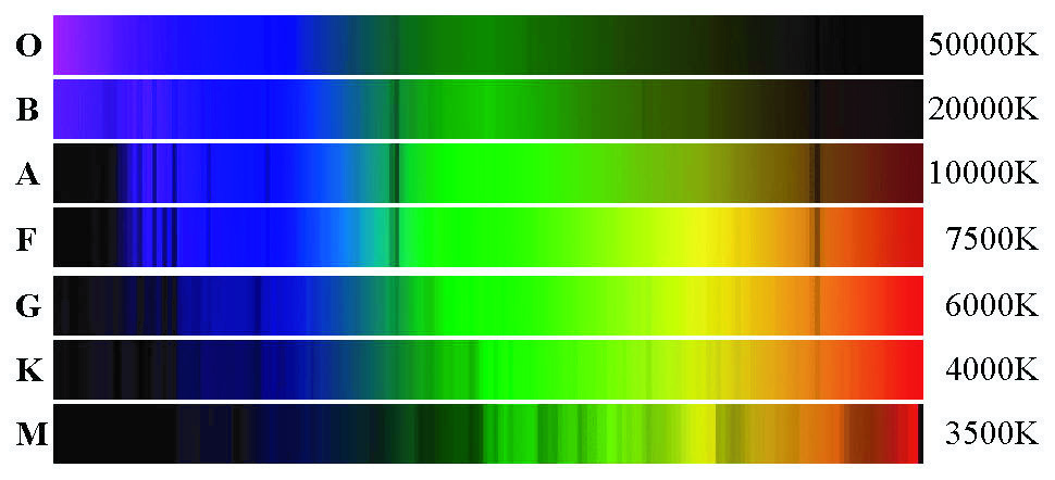
3.Color or \Spectrum": Our perception of light in three primary colors comes
from the di
erent sensitivity of receptors in our eyes to light in distinct wave-
length ranges within the visible spectrum, corresponding to Red, Green, and
Blue (RGB). Similarly, in astronomy, the light from a star is often passed
through di
erent sets of
lters designed to transmit only light within some
characteristic band of wavelengths, for example the UBV (Ultraviolet, Blue,
Visible)
lters that make up the so-called \Johnson photometric system". But
much more information can be gained by using a prism or (more commonly) a
di
raction grating to split the light into its spectrum, de
ning the variation in
wavelength of the
ux,F, by measuring its value within narrow wavelength
bins of width
. The \spectral resolution" =available depends on
the instrument (spectrometer) as well as the apparent brightness of the light
source, but for bright stars with modern spectrometers, the resolution can be
10,000 or more, or indeed, for the Sun, many millions. As discussed below,
a key reason for seeking such high spectral resolution is to detect \spectral
lines" that arise from the absorption and emission of radiation via transitions
between discrete energy levels of the atoms within the star. Such spectral lines
1.2 Scales and Orders of Magnitude 5
can provide an enormous wealth of information about the composition and
physical conditions in the source star.
Indeed, a key theme here is that these 3 apparently rather limited observational
properties of point-stars { position, apparent brightness, and color spectrum {
can, when combined with a clear understanding of some basic physical principles,
allow us to infer many of the key physical properties of stars, for example:
1.Distance
2.Luminosity
3.Temperature
4.Size (i.e. Radius)
5.Elemental Composition (denoted as X,Y,Z for mass fraction of H, He, and
of heavy \metals")
6.Velocity (Both radial (toward/away) and transverse (\proper motion" across
the sky)
7.Mass (and surface gravity )
8.Age
9.Rotation (PeriodPand/or equatorial rotation speed Vrot)
10.Mass loss properties (e.g., rate _Mand out
ow speed V)
11.Magnetic
eld
These are ranked roughly in order of diculty for inferring the physical prop-
erty from one or more of the three types of observational data. It also roughly
describes the order in which we will examine them below. In fact, except for
perhaps the last two, which we will likely discuss only brie
y if at all (though
they happen to be two specialities of my own research), a key goal is to provide a
basic understanding of the combination of physical theories, observational data,
and computational methods that make it possible to infer each of the
rst 9
physical properties, at least for some stars.
1.2 Scales and Orders of Magnitude
Scales and Orders of Magnitude
- The text outlines a pedagogical approach to understanding stellar properties through physical theories, observational data, and computational methods.
- A geometric progression using powers of ten is employed to bridge the gap between human scales and the vastness of the universe.
- The scale of the Earth is seven orders of magnitude larger than a human, while the Sun is approximately one hundred times the diameter of Earth.
- Distances in the solar system are often measured in light-travel time, with the Sun being eight light minutes away from Earth.
- Interstellar distances represent a massive jump in scale, with the nearest star being five orders of magnitude further than the Earth-Sun distance.
- The Milky Way galaxy, containing 100 billion stars, extends the cosmic scale another five orders of magnitude beyond the distance between individual stars.
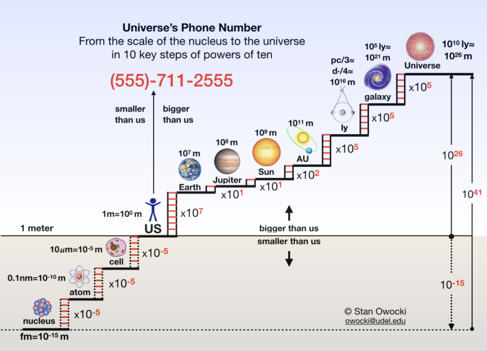
As a mneumonic, this is cast as a 10-digit "telephone number", with the 3-digit "area code" representing the 3 steps of 10-5 from us down to the nucleus, and 7-digit main-number representing 7 key steps to the scale of the universe.
These are ranked roughly in order of diculty for inferring the physical prop-
erty from one or more of the three types of observational data. It also roughly
describes the order in which we will examine them below. In fact, except for
perhaps the last two, which we will likely discuss only brie
y if at all (though
they happen to be two specialities of my own research), a key goal is to provide a
basic understanding of the combination of physical theories, observational data,
and computational methods that make it possible to infer each of the
rst 9
physical properties, at least for some stars.
1.2 Scales and Orders of Magnitude
Before proceeding, let us make a brief aside to discuss ways to get our heads
around the enormous scales we encounter in astrophysics.
As illustrated in
gure 1.1, one approach is to use a geometric progression
through powers of ten1, from the scale from our own bodies, which in standard
metric (MKS) units is of order 1 meter (m), to the progressively larger scales in
our universe.
For example, the meter itself was originally de
ned (in 1793!) as one ten mil-
lionth, or 10�7, of the distance from Earth's equator to poles; this thus means
1There are many online versions, including a rather dated (1977) but still informative movie
titled \Powers of Ten", which you can readily
nd by google; for a modern version, see
http://www.htwins.net/scale2/.
6 Introduction
Figure 1.1 Graphic to illustrate key powers-of-ten steps between our own human scale
of 1 meter, both upward to the scale of the universe (1026m), and also downward to
the scale of an atomic nucleus (10�15m). As a mneumonic, this is cast as a 10-digit
\telephone number", with the 3-digit \area code" representing the 3 steps of 10�5
from us down to the nucleus, and 7-digit main-number representing 7 key steps to the
scale of the universe.
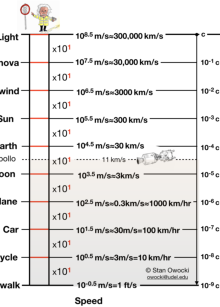
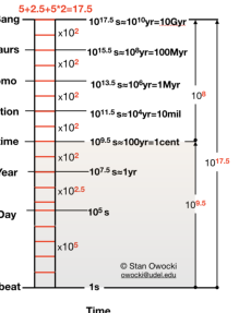
Figure 1.2 Graphics to illustrate the range of scales for time (left) and speed (right).
a total of seven steps in powers of ten from the scale of us to that of our Earth.
1.2 Scales and Orders of Magnitude 7
This is the largest scale for which most of us have direct experience, e.g., from
overseas plane travel, or a cross country drive.
The other, rocky inner planets are somewhat smaller but same order as Earth;
among the outer, gas giant planets Jupiter is the largest, about a factor ten
larger than Earth, while the Sun is about another factor ten larger still, with a
diameterD
1:4106km, about a factor hundred bigger than Earth, or of
order 109m.
The Earth-Sun distance, dubbed an \astronomical unit" (AU), is about about
a hundred solar diameters, at 150 million km. This is of order 108km = 1011m,
or four further powers of ten beyond the scale of our Earth, and so a total of
eleven orders of magnitude bigger in scale than our own bodies.
An alternative way to characterize this is in terms of the time it takes light,
which propagates at a speed c= 300;000 km/s, to reach us from the Sun; a simple
calculation gives t=d=c= 1:5e8=3e5 = 500 s, which is about eight minutes; so
we can say the Sun is 8 light minutes from Earth.
By contrast, it takes light from the next nearest star, Proxima Centauri, about
four years to reach us, meaning it is at a distance of 4 light years (ly). A simple
calculation shows that one year is 1 yr = 365 2460603107s; so
multiplying by the speed of light c= 3105km/s gives that 1 ly 91012km,
or of order 1016m. Thus the scale between the stars is another
ve order of
magnitude greater than that the Earth-Sun distance, or sixteen orders greater
than that of ourselves.
The Sun is only one of about 100 billion (1011) stars in our Milky Way galaxy,
a disk that is about 1000 ly thick, and about 100,000 ly across. Thus our galaxy is
another
ve orders of magnitude bigger than the scale between individual stars,
Scales of the Universe
- The distance between stars is roughly 10 to the 16th power meters, which is five orders of magnitude greater than the Earth-Sun distance.
- The Milky Way galaxy is a disk 100,000 light-years across, representing another five-order jump in scale to 10 to the 21st power meters.
- The observable universe spans 26 orders of magnitude from the human scale, reaching approximately 10 to the 26th power meters.
- A '10-digit phone number' mnemonic (555-711-2555) maps the powers of ten from atomic nuclei up to the entire universe.
- Time and speed scales are equally vast, ranging from a single human heartbeat to the 14-billion-year age of the universe and the speed of light.
The full sequence of steps over this span thus looks something like a 10-digit phone number with area code: 555-711-2555.
calculation shows that one year is 1 yr = 365 2460603107s; so
multiplying by the speed of light c= 3105km/s gives that 1 ly 91012km,
or of order 1016m. Thus the scale between the stars is another
ve order of
magnitude greater than that the Earth-Sun distance, or sixteen orders greater
than that of ourselves.
The Sun is only one of about 100 billion (1011) stars in our Milky Way galaxy,
a disk that is about 1000 ly thick, and about 100,000 ly across. Thus our galaxy is
another
ve orders of magnitude bigger than the scale between individual stars,
or about 1021m, thus twenty-one orders bigger than us.
The universe itself is about 14 billion years old (14 Gyr), meaning that the
most distant galaxies we can see are of order 1010ly1026m away. We thus
see that twenty-six powers of ten takes us from our own scale to the scale of the
entire observable universe!
To recap, powers of ten steps of 7 takes us from us to the Earth; then powers
of ten steps 1, 1 and 2 takes us from Earth to the size of Jupiter, Sun, and Earth-
Sun distance. Then 3 successive power-ten steps of 5 take us to the distance of
the nearest other star; to the size of our galaxy; and
nally to the size of the
universe. It can be helpful to remember this 711-2555 rule as a mnemonic { like
a 7-digit telephone number { to capture the progression between key scales that
characterize our place in the universe.
Indeed, we can extend this even to small scales, by noting that 5 powers of ten
smaller takes us successively to the characteristic size of cell, 10�5m=10 micron;
then to the size of atoms, 10�10m = 0.1 nanometer; and
nally to the scale of an
atomic nucleus,10 femtometer (a.k.a. \fermi") or 1 fm = 10�15m.
The full sequence of steps over this span thus looks something like a 10-digit
phone number with area code: 555-711-2555, representing the power of ten steps
from scales of nuclei to atoms to cells to us to Earth to Jupiter to Sun to au
8 Introduction
(distance to Sun) to light-year ( distance between stars) to our Galaxy to the
Universe.
Finally, the enormous timescales at play in the universe can likewise be dicult
to grasp.
As illustrated in the left panel of
gure 1.2, humans experience time in our
everyday world on the scale of a second, which is roughly the order of a single
heartbeat. We live a maximum of about 100 years, or about 3 billion seconds . In
comparison, it is estimated that the Earth is about 4.4 billion years old, almost
as old as the Sun and the rest of the solar system. The Sun is expected to sustain
its current energy output for about another 5 billion years, and so have a full
lifetime of about 10 billion years. And as discussed below (see x8), the lifetimes
of other stars can depend strongly on their mass; the most massive stars (about
a hundred solar masses) live only about ten million years, while those with mass
less than the Sun are expected to last for up to hundred billion years, much much
longer than the current age of the universe!
The right panel of
gure 1.2 gives a similar graphic for the range of speeds,
from our own slow walk, through others (bicycles, cars, airplanes) we experience,
then ranging to speeds of the moon, earth and Sun in their orbits, to stellar winds
and supernovae, and
nally ending with the maximum possible speed, the speed
of light,c= 3108m/s. The right axis relates the fraction of the light speed for
each of the progression of nine powers from walking to light itself.
The remaining sections below explain how we are able to discover these fun-
damental properties of stars, beginning with their distance.
1.3 Questions and Exercises 9
1.3 Questions and Exercises
Do the following computations by hand (without a calculator), to obtain results
good to just one or two signi
cant
gures, but clearly showing the correct order
of magnitude.
Quick Question 1:
Inferring Distances and Angular Size
- The text introduces fundamental astronomical calculations involving the speeds of Earth's rotation, its orbit around the Sun, and the Sun's orbit within the Milky Way.
- It provides exercises for calculating distances and travel times using light-seconds, solar radii, and astronomical units (AU).
- The concept of angular size is introduced as a primary method for intuitively and mathematically estimating the distance of an object.
- The small-angle approximation is explained, showing how the tangent and sine functions simplify to a linear relationship for distant objects.
- Geometric formulas are established to relate an object's physical size and its distance to the angle it subtends in a viewer's field of vision.
The apparent angular size that object subtends in our overall field of view is then used intuitively by our brains to infer the object's distance, based on our extensive experience that a greater distance makes the object subtend a smaller angle.
of light,c= 3108m/s. The right axis relates the fraction of the light speed for
each of the progression of nine powers from walking to light itself.
The remaining sections below explain how we are able to discover these fun-
damental properties of stars, beginning with their distance.
1.3 Questions and Exercises 9
1.3 Questions and Exercises
Do the following computations by hand (without a calculator), to obtain results
good to just one or two signi
cant
gures, but clearly showing the correct order
of magnitude.
Quick Question 1:
a. What speed does a person at the equator move due to Earth's rotation? Give your
answer in mi/hr, km/hr, and m/s.
b. What is the speed of the Earth in its orbit around the Sun? Give your answer in
AU/yr, km/s, mi/hr, and in terms of the fraction of the speed of light vorb=c?
c. The Sun is about 25,000 ly from the center of the Milky Way, and takes about 200
million years to complete one \Galactic year". What is the speed of Sun in its orbit
around the Milky Way, in km/s. In ly/yr? In terms of the fraction of the speed of light
vorb=c?
Quick Question 2: The Sun has a radius of about 700,000 km.
a. How many solar radii in 1 AU? In 1 ly?
b. How many Earth radii REin one solar radius R
?
c. Solar neutrinos created in the Sun's core travel at very nearly speed of light but
hardly interact with solar matter. How long does it take such core neutrinos to reach
the solar surface? How long to reach us on Earth?
d. What then is the solar radius in light-seconds?
Quick Question 3: The Moon is about 240,000 miles from Earth.
a. What is the Earth-Moon distance in km? In light-seconds? In Earth radii RE? In
solar radiiR
?
b. How many Earth-Moon distances in 1 AU?
2 Inferring Astronomical Distances
2.1 Angular size
To understand ways we might infer stellar distances, let's
rst consider how
we intuitively estimate distance in our everyday world. Two common ways are
through apparent angular size , and/or using our stereoscopic vision .
For the
rst, let us suppose we have some independent knowledge of the phys-
ical size of a viewed object. The apparent angular size that object subtends in
our overall
eld of view is then used intuitively by our brains to infer the object's
distance, based on our extensive experience that a greater distance makes the
object subtend a smaller angle.
s α AB
Cd
Figure 2.1 Angular size and parallax: The triangle illustrates how an object of
physical size s(BC) subtends an angular size
when viewed from a point A that is
at a distance d. Note that the same triangle can also illustrate the parallax angle
toward the point A at distance dwhen viewed from two points B and C separated by
a lengths.
As illustrated in
gure 2.1, we can, with the help of some elementary geometry,
formalize this intuition to write the speci
c formula. The triangle illustrates
the angle
subtended by an object of size sfrom a distance d. From simple
trigonometry, we
nd
tan(
=2) =s=2
d: (2.1)
For distances much larger than the size, d
s, the angle is small,
1,
for which the tangent function can be approximated (e.g. by
rst-order Tay-
lor expansion) to give tan(
=2)
=2, where
is measured here in radians.
2.1 Angular size 11
(1 rad = (180 =)57). The relation between distance, size, and angle thus
becomes simply
s
d: (2.2)
Of course, if we know the physical size and then measure the angular size, we
can solve the above relation to determine the distance d=s=
.
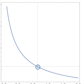
0.20.611.40.511.52Tan x
Sin xx
xx+x3/3
x-x3/6
Figure 2.2 Taylor expansion of trig functions sin xand tanx, aboutx= 0 to order x
and orderx3.
dR
RαAB
Csin(α/2)=R/d
for R<<D , α≈2R/d
Figure 2.3 Diagram to illustrate the relation between angular size
and diameter 2 R
for a sphere at distance d.
As illustrated in
gure 2.3, for a spherical object the angular size
is related
to the distance dand radius Rthrough the sine function,
sin(
=2) =R=d: (2.3)
From
Measuring the Cosmos
- The distance to a celestial object can be calculated by comparing its known physical size to its observed angular size.
- Small-angle approximations simplify complex trigonometric relations into linear equations for distant astronomical bodies.
- Atmospheric seeing blurs images to about 1 arcsecond, preventing ground-based telescopes from resolving the tiny angular diameters of most stars.
- Trigonometric parallax mimics human stereoscopic vision by using two different viewpoints to perceive depth and distance.
- The parallax effect is inversely proportional to distance, meaning closer objects exhibit a larger shift in apparent position.
Neurosensors in the eye muscles that effect this inward pointing relay this inward angle to our brain, where it is processed to provide our sense of 'depth' perception.
Of course, if we know the physical size and then measure the angular size, we
can solve the above relation to determine the distance d=s=
.
0.20.611.40.511.52Tan x
Sin xx
xx+x3/3
x-x3/6
Figure 2.2 Taylor expansion of trig functions sin xand tanx, aboutx= 0 to order x
and orderx3.
dR
RαAB
Csin(α/2)=R/d
for R<<D , α≈2R/d
Figure 2.3 Diagram to illustrate the relation between angular size
and diameter 2 R
for a sphere at distance d.
As illustrated in
gure 2.3, for a spherical object the angular size
is related
to the distance dand radius Rthrough the sine function,
sin(
=2) =R=d: (2.3)
From
gure 2.2 we see that, for the small angles that apply at large distances
d
R, this again reduces to a simple linear form,
2R=d, that relates size
to distance.
12 Inferring Astronomical Distances
For example, the distance from the Earth to the Sun, known as an \astronom-
ical unit" (abbreviated \au"), is d= 1 au150106km, much larger than the
Sun's physical size (i.e. diameter), which is about s= 2R
1:4106km. This
means that the Sun has an apparent angular diameter of
2R
1au0:009 rad0:5= 30 arcmin = 1800 arcsec : (2.4)
However, as noted in x1.2 (and illustrated in
gure 1.1), even the nearest stars
are more than 200,000 times further away than the Sun. If we assume a similar
physical radius (which actually is true for one of the components of the nearest
star system,
Centauri A), then
=2R
200;000au0:009 arcsec: (2.5)
For ground-based telescopes, the distorting e
ect of the Earth's atmosphere,
known as \atmospheric seeing" (see x13.2), blurs images over an angle size of
about 1 arcsec, making it very dicult to infer the actual angular size. There are
some specialized techniques, e.g. \speckle interferometry", that can just barely
resolve the angular diameter of a few nearby giant stars (e.g. Betelgeuse, a.k.a.
Ori). But generally the diculty of measuring a star's angular size means that,
even if we knew its physical size, we can not use this angular-size method to infer
its distance.
2.2 Trignonometric parallax
Fortunately, there is a practical, quite direct way to infer distances to at least
relatively nearby stars, namely through the method of trigonometric parallax .
This is physically quite analogous to the stereoscopic vision by which we use
our two eyes to infer distances to objects in our everyday world. To understand
this parallax e
ect, we can again refer to
gure 2.1. If we now identify sas the
separation between the eyes, then when we view objects at some nearby distance
d, the two eyes, in order to combine the separate images as one, have to point
inward an angle
= 2 arctan( s=2d). Neurosensors in the eye muscles that e
ect
this inward pointing relay this inward angle to our brain, where it is processed
to provide our sense of \depth" (i.e. distance) perception.
You can easily experiment with this e
ect by placing your
nger a few inches
from your face, then blinking between your left and right eye, which thus causes
the image of your
nger to jump back a forth by the angle
= 2 arctan( s=2d).
The eye separation sis
xed, but as you move the
nger closer and further away,
the angle shift will become respectively larger and smaller.
Home Experiment: To illustrate this close link between parallax and angular size,
try the following experiment. In front of a wall mirror, close one eye and then extend
a
nger from either arm to the mirror, covering the image of your closed eye. Without
moving your
nger, now switch the closure to the other eye. Note that the
nger has
2.2 Trignonometric parallax 13
also switched to cover the other (now closed) eye, even though you didn't physically
move it! Note further that this even still works as you decrease the distance from your
face to the mirror. The key point here is that the \parallax" angle shift of your
nger,
which results from switching perspective from one eye to the other, exactly
ts the
Trigonometric Parallax and Stellar Distance
- Trigonometric parallax uses a change in perspective to calculate the distance of an object based on an angular shift.
- While human binocular vision is limited to about 10 meters, larger baselines allow for the measurement of astronomical distances.
- Early 19th-century astronomers used the Earth's diameter as a baseline to calculate the distance to Mars during opposition.
- Stellar parallax utilizes the Earth's orbital radius (1 AU) as a baseline, observing stars at six-month intervals to maximize the shift.
- The 'parsec' is defined as the distance at which a star exhibits a parallax angle of one arcsecond, equivalent to roughly 3.26 light-years.
- Atmospheric blurring and the tiny scale of parallax angles (all less than one arcsecond) make these measurements extremely challenging.
The key point here is that the parallax angle shift of your finger, which results from switching perspective from one eye to the other, exactly fits the apparent angular separation between your own mirror-image eyes.
nger from either arm to the mirror, covering the image of your closed eye. Without
moving your
nger, now switch the closure to the other eye. Note that the
nger has
2.2 Trignonometric parallax 13
also switched to cover the other (now closed) eye, even though you didn't physically
move it! Note further that this even still works as you decrease the distance from your
face to the mirror. The key point here is that the \parallax" angle shift of your
nger,
which results from switching perspective from one eye to the other, exactly
ts the
apparent angular separation between your own mirror-image eyes.
Of course, for distances much more than the separation between our eyes,
d
s, the angle becomes too small to perceive, and so we can only use this
approach to infer distances of about, say, 10 m. But if we extend the baseline
to much larger sizes s, then when coupled with accurate measures of the angle
shift
, this method can be used to infer much larger distances.
For example, in the 19th century, there were e
orts to use this approach to
infer the distance to Mars at time when it was relatively close to Earth, namely
at opposition (i.e. when Mars is on the opposite side of the Earth from the Sun).
Two expeditions tried to measure the position of Mars at the same time from
widely separated sites on Earth. If the distance between the sites is known, the
angle di
erence in the measured directions to Mars, which turns out to be about
an arcmin, yields a distance to Mars.
The largest separation possible from two points on the surface of the Earth
is limited by the Earth's diameter. But to apply this method of trigonometric
parallax to infer distances to stars, we need to use a much bigger baseline than
the Earth's diameter. Fortunately though, we don't need then to go into space.
au
Jan.dJuly
*p*
**
nearby
stard/pc = arcsec/pbackground stars *
***
****
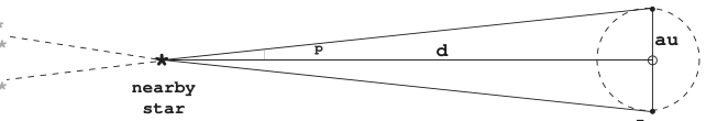
Figure 2.4 Illustration of stellar parallax, in which a relatively nearby star appears to
shift against background stars by a parallax angle pas the earth moves through the 1
au radius of earth's orbit. The distance din parsec (pc) is given by the inverse of p
measured in arcsec.
As illustrated in
gure 2.4, just waiting a half year from one place on the Earth
allows us, as a result of the Earth's orbit around the Sun, to view the stars from
two points separated by twice the Earth's orbital radius, i.e. 2 au. By convention,
however, the associated \parallax angle"
of a star is traditionally quoted in
terms of the shift from a baseline sof just oneau. If we scale the parallax angle
in units of an arcsec, the distance is
d=s
=206;265 arcsec=radian
=radianauarcsec
parsec; (2.6)
14 Inferring Astronomical Distances
where we note that the conversion between arcsec and radian is given by (180/ )
degree/radian60 arcmin/degree 60 arcsec/arcmin = 206,265 arcsec/radian.
In the last equality, we have also introduced the distance unit parsec (short for
\parallax second", and often further abbreviated as \pc"), which is de
ned as
the distance at which the parallax angle is 1 arcsec. It is thus apparent that
1 pc = 206;265 au, which works out to give 1 pc 31016m.
The \parsec" is one of the two most common units used to characterize the
huge distances we encounter in astronomy. The other is the light-year , which is
the distance light travels in a year, at the speed of light c= 3108m/s. The
number of seconds in a year is given by 1 yr = 365 246060 = 3:15107s,
which, coincidentally, can be remembered as 1 yr 107s (or sincep
103:16,
1 yr107:5s). Thus a light-year is roughly 1 ly 3108+79:51015
1016m. In terms of parsecs, we can see that 1 pc 3:26 ly.
The parallax for even the nearest star is less than an arcsec, implying stars are
all at distances more (generally much more) than a parsec. By repeated observa-
tion, the roughly 1 arcsec overall blurring of single stellar images by atmospheric
Measuring Cosmic Distances
- The parsec and light-year are the primary units for astronomical distance, with one parsec equaling approximately 3.26 light-years.
- Ground-based parallax measurements are limited to about 100 parsecs due to atmospheric blurring, though averaging techniques can improve accuracy.
- Space-based missions like Hipparchus and Gaia significantly extend our reach by measuring parallax angles down to a milliarcsecond.
- The Astronomical Unit (au) serves as the fundamental baseline for all stellar distance calculations.
- Modern radar ranging of planets like Venus allows for the precise trigonometric derivation of the au's physical length.
- Solid angle, measured in steradians, provides a two-dimensional generalization for describing the size of extended objects in the sky.
The parallax for even the nearest star is less than an arcsec, implying stars are all at distances more (generally much more) than a parsec.
the distance at which the parallax angle is 1 arcsec. It is thus apparent that
1 pc = 206;265 au, which works out to give 1 pc 31016m.
The \parsec" is one of the two most common units used to characterize the
huge distances we encounter in astronomy. The other is the light-year , which is
the distance light travels in a year, at the speed of light c= 3108m/s. The
number of seconds in a year is given by 1 yr = 365 246060 = 3:15107s,
which, coincidentally, can be remembered as 1 yr 107s (or sincep
103:16,
1 yr107:5s). Thus a light-year is roughly 1 ly 3108+79:51015
1016m. In terms of parsecs, we can see that 1 pc 3:26 ly.
The parallax for even the nearest star is less than an arcsec, implying stars are
all at distances more (generally much more) than a parsec. By repeated observa-
tion, the roughly 1 arcsec overall blurring of single stellar images by atmospheric
seeing can be averaged to give a position accuracy of about
0:01 arcsec,
implying that one can estimate distances to stars out to about d100 pc. The
Hipparchus satellite orbiting above Earth's atmosphere can measure parallax an-
gles approaching a milliarcsec (1 mas = 10�3arcsec), thus potentially extending
distance measurements for stars out to about a kiloparsec, d1 kpc. However,
parallax measurements out to such distances typically require a relatively bright
source. In practice, only a fraction of all the stars (those with the highest intrin-
sic brightness, or \luminosity") with distances near d1 kpc have thus far had
accurate measurements of their parallax1.
Again, from the above discussion it should be apparent that parallax is really
the \
ip slide" of the angular size vs. distance relation. That is, the triangle in
gure 2.1 was initially used to illustrate how, from the perspective of a given
point A, the angle
subtended by an object is set by the ratio of its size sto its
distanced. But if we consider a simple change of observer's perspective to the
two endpoints (B and C) of the size seqment s, then the same triangle can be
used equally well to illustrate the observed parallax angle
for the point A at a
distanced.
For the large ( >parsec) distances in astronomy, it is convenient to rewrite
our simple equation (2.2) to scale angular size in arcsec, with the size in au and
distance in pc:
arcsec=s=au
d=pc: (2.7)
1Since 2013 a follow-up satellite mission call Gaia has been in the process of measuring the
absolute position and parallax to roughly one billion stars; see http://sci.esa.int/gaia/.
2.3 Determining the Astronomical Unit (au) 15
2.3 Determining the Astronomical Unit (au)
We thus see that determining the distance of the Earth to the Sun, i.e. measuring
the physical length of an au, provides a fundamental basis for determining the
distances to stars and other objects in the universe. In modern times, one way this
is computed involves
rst measuring the distance from the Earth to the planet
Venus through \radar ranging", i.e. measuring the time tit takes a radar signal
to bounce o
Venus and return to Earth. The associated Earth-Venus distance
is then given by
dEV=ct
2: (2.8)
If this distance is measured at the time when Venus has its \maximum elonga-
tion", or maximum angular separation, from the Sun, which is found to be about
47o, then one can use simple trigonometry to derive a physical value of the au.
The details are left as an exercise for the reader. (See Exercise 2-1 at the end of
this section.)
2.4 Solid angle
In general objects that have a measurable angular size on the sky are extended
intwoindependent directions. As the 2D generalization of an angle along just
one direction, it is useful then to de
ne for such objects a 2D solid angle
,
measured now in square radians , but more commonly referred by the shorthand
\steradians ".
Just as projected area Ais related to the square of physical size s(or radius
R), so is solid angle
related to the square of the angular size
Solid Angles and Celestial Geometry
- The distance to Venus at maximum elongation can be used with simple trigonometry to calculate the physical value of an astronomical unit (au).
- Solid angle is introduced as the two-dimensional generalization of an angle, measured in steradians or square radians.
- The solid angle of an object is mathematically defined as the ratio of its projected area to the square of its distance.
- A full sphere contains 4π steradians, which is equivalent to approximately 41,253 square degrees.
- The Sun and Moon each cover a solid angle of about 0.2 square degrees, representing only 1/200,000th of the total sky.
- Calculations of solid angles help explain physical phenomena, such as why the full moon is significantly dimmer than the sun.
Integration over a full sphere shows that there are 4π steradians in the full sky.
If this distance is measured at the time when Venus has its \maximum elonga-
tion", or maximum angular separation, from the Sun, which is found to be about
47o, then one can use simple trigonometry to derive a physical value of the au.
The details are left as an exercise for the reader. (See Exercise 2-1 at the end of
this section.)
2.4 Solid angle
In general objects that have a measurable angular size on the sky are extended
intwoindependent directions. As the 2D generalization of an angle along just
one direction, it is useful then to de
ne for such objects a 2D solid angle
,
measured now in square radians , but more commonly referred by the shorthand
\steradians ".
Just as projected area Ais related to the square of physical size s(or radius
R), so is solid angle
related to the square of the angular size
. For an object
at a distance dwith projected area A, the solid angle is just
=A
d2R2
d2=
2; (2.9)
where the latter equalities assume a sphere (or disk) with projected radius R
and associated angular radius
=R=d.
For more general shapes,
gure 2.5 illustrates how a small solid-angle patch
is de
ned in terms of ranges in the standard spherical angles representing
co-latitude and azimuth
on a sphere. An extended object would then have a
solid angle given by the integral
=Z
d
sind: (2.10)
Integration over a full sphere shows that there are 4steradians in
the full sky. This represents the 2D analog to the 2 radians around the full
circumference of a circle.
For our example of a circular patch of angular radius
, let us assume the
16 Inferring Astronomical Distances
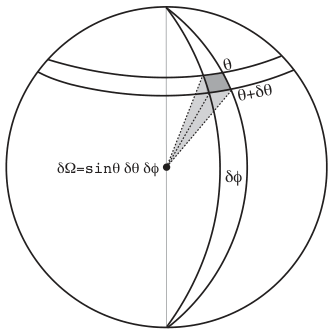
θ
θ+δθ
δφ δΩ=sinθ δθ δφ
Figure 2.5 Diagram to illustrate a small patch of solid angle
seen by an observer at
the center of a sphere, with size de
ned by ranges in the co-latitude and azimuth
.
object is centered around the coordinate pole { representing perhaps the image
of a distant spherical object like the Sun or moon. The azimuthal symmetry
means the
integral evaluates to 2 , while carrying out the remaining integral
over co-latitude range 0 to
then gives
= 2[1�cos
]: (2.11)
In particular, applying the angular radius of the Sun
R
=au and expanding
the cosine to
rst order (i.e., cos x1�x2=2), we
nd
= 2[1�cos(R
=au)](R
=au)2
2
: (2.12)
One can alternatively measure solid angle in terms of square degrees. Since
there are 180 =57:3 degrees in a radian, there are (180 =)2= 57:323283
square degrees in a steradian; the number of square degrees in the 4 steradians
of the full sky is thus
4180
2
= 41;253 deg2: (2.13)
The Sun and moon both have angular radii of about 0 :25o, meaning they each
have a solid angle of about (0:25)2==16 = 0:2 deg2= 610�5ster, which
is about 1=200;000 of the full sky2.
2.5 Questions and Exercises
Quick Question 1: A helium party balloon of diameter 20 cm
oats 1 meter above
your head.
2If you think about it, you'll see that this helps explain why a full moon is about a million
times dimmer than full sunlight! See Exercise 2-3.
2.5 Questions and Exercises 17
a. What is its angular diameter, in degrees and radians?
b. What is its solid angle, in square degrees and steradians?
c. What fraction of the full sky does it cover?
d. At what height hwould its angular diameter equal that of the Moon and Sun?
Quick Question 2:
a. What angle
would the Earth-Sun separation subtend if viewed from a distance
ofd= 1 pc? Give your answer in both radian and arcsec.
b. How about from a distance of d= 1 kpc?
Quick Question 3: Over a period of several years, two stars appear to go around each
other with a
xed angular separation of 1 arcsec.
a. What is the physical separation, in au, between the stars if they have a distance
d= 10 pc from Earth?
b. If they have a distance d= 100 pc?
Exercise 1: At the time when Venus exhibits its maximum elongation angle of about
Luminosity and Distance Measurement
- The text provides practical exercises for calculating astronomical distances using angular separation, radar timing, and parallax errors.
- Apparent brightness is defined as the flux of light, which is the energy per unit time per unit area captured by a detector.
- The inverse-square law dictates that light intensity decreases in proportion to the square of the distance as energy spreads over a spherical area.
- The 'Standard Candle' method allows astronomers to calculate distance by comparing an object's known intrinsic luminosity to its observed flux.
- When distance is known via trigonometric parallax, the same physical relationship is used to calculate a star's total power output or luminosity.
This is a profoundly important equation in astronomy, and so you should not just memorize it, but embed it completely and deeply into your psyche.
would the Earth-Sun separation subtend if viewed from a distance
ofd= 1 pc? Give your answer in both radian and arcsec.
b. How about from a distance of d= 1 kpc?
Quick Question 3: Over a period of several years, two stars appear to go around each
other with a
xed angular separation of 1 arcsec.
a. What is the physical separation, in au, between the stars if they have a distance
d= 10 pc from Earth?
b. If they have a distance d= 100 pc?
Exercise 1: At the time when Venus exhibits its maximum elongation angle of about
47ofrom the Sun, a radar signal is found to take a round trip time t= 667 sec to
return to Earth. Assuming both Earth and Venus have circular orbits, and using the
speed of light c= 3105km/s, compute (in km) the Earth-Sun distance, 1 AU.
Exercise 2: With a suciently large telescope in space, with angle error
1 mas,
for how many more stars can we expect to obtain a measured parallax than we can
from ground-based surveys with
20 mas? (Hint: What assumption do you need
to make about the space density of stars in the region of the galaxy within 1 kpc from
the Sun/Earth?)
Exercise 3: a. Assuming the Moon re
ects a fraction a(dubbed the \albedo") of
sunlight hitting it, derive an expression for the ratio of apparent brightness ( Fmoon=F
)
between the full Moon and Sun, in terms of the Moon's radius Rmoon and its distance
from earth, dem
au. b. Derive the value of the albedo afor which this ratio equals
the fraction of sky subtended by the Moon's solid angle, i.e. for which Fmoon=F
=
moon=4.
3 Inferring Stellar Luminosity
3.1 \Standard Candle" methods for distance
In our everyday experience, there is another way we sometimes infer distance,
namely by the change in apparent brightness for objects that emit their own light,
with some known power or \luminosity". For example, a hundred watt light bulb
at a distance of d= 1 m certainly appears a lot brighter than that same bulb at
d= 100 m. Just as for a star, what we observe as apparent brightness is really
a measure of the
uxof light, i.e. energy per unit time per unit area (erg/s/cm2
in CGS units, or watt/m2in MKS).
When viewing a light bulb with our eyes, it's just the rate at which the light's
energy is captured by the area of our pupils. If we assume the light bulb's emission
isisotropic (i.e., the same in all directions), then as the light travels outward to
a distanced, its power or luminosity is spread over a sphere of area 4 d2. This
means that the light detected over a
xed detector area (like the pupil of our
eye, or, for telescopes observing stars, the area of the telescope mirror) decreases
in proportion to the inverse-square of the distance, 1 =d2. We can thus de
ne the
apparent brightness in terms of the
ux,
F=L
4d2: (3.1)
This is a profoundly important equation in astronomy, and so you should not
just memorize it, but embed it completely and deeply into your psyche.
In particular, it should become obvious that this equation can be readily used
to infer the distance to an object of known luminosity , an approach called the
standard candle method. (Taken from the idea that a candle, or at least a \stan-
dard" candle, has a known luminosity or intrinisic brightness.) As discussed
further in sections below, there are circumstances in which we can get clues to
a star's (or other object's) intrinsic luminosity L, for example through careful
study of a star's spectrum. If we then measure the apparent brightness (i.e.
ux
F), we can infer the distance through:
d=r
L
4F: (3.2)
Indeed, when the study of a stellar spectrum is the way we infer the luminos-
3.2 Intensity or Surface Brightness 19
ity, this method of distance determination is sometimes called \spectroscopic
parallax".
Of course, if we can independently determine the distance through the actual
trigonometric parallax, then such a simple measurement of the
ux can instead
be used to determine the luminosity,
L= 4d2F: (3.3)
Stellar Luminosity and Surface Brightness
- Luminosity can be determined through spectroscopic parallax by measuring a star's spectrum and apparent brightness.
- The Sun's luminosity is approximately 4 x 10^26 Watts, a scale equivalent to four million billion billion 100-watt light bulbs.
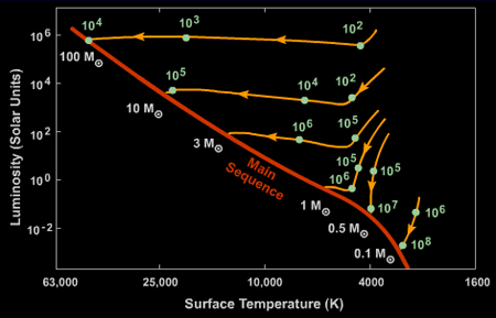
- Solar luminosity serves as a benchmark for other stars, which range from 1/1000th to one million times the Sun's power.
- Surface brightness, or specific intensity, is a unique quantity that remains constant regardless of the observer's distance from the object.
- While the flux of light decreases with distance, the solid angle it occupies shrinks proportionally, keeping the ratio of flux per solid angle stable.
- The surface brightness of the Sun viewed from Earth is identical to the brightness one would experience standing on the Sun's surface.
Thus we see that the Sun emits the power of about 4 x 10^24 100-watt light bulbs! In common language this corresponds to four million billion billion, a number so huge that it loses any meaning.
study of a star's spectrum. If we then measure the apparent brightness (i.e.
ux
F), we can infer the distance through:
d=r
L
4F: (3.2)
Indeed, when the study of a stellar spectrum is the way we infer the luminos-
3.2 Intensity or Surface Brightness 19
ity, this method of distance determination is sometimes called \spectroscopic
parallax".
Of course, if we can independently determine the distance through the actual
trigonometric parallax, then such a simple measurement of the
ux can instead
be used to determine the luminosity,
L= 4d2F: (3.3)
In the case of the Sun, the
ux measured at Earth is referred to as the \solar
constant", with a measured mean value of about
F
1:4kW
m2= 1:4106erg
cm2s: (3.4)
If we then apply the known mean distance of the Earth to the Sun, d= 1 au, we
obtain for the solar luminosity
L
41026W = 41033erg
s: (3.5)
Thus we see that the Sun emits the power of about 4 1024100-watt light bulbs!
In common language this corresponds to four million billion billion, a number so
huge that it loses any meaning. It illustrates again how in astronomy we have to
think on a entirely di
erent scale than we are used to in our everyday world.
But once we get used to the idea that the luminosity and other properties of
the Sun are huge but still
nite and measurable, we can use these as benchmarks
for characterizing analogous properties of other stars and astronomical objects.
In the case of stellar luminosities, for example, these typically range from about
L
=1000 for very cool, low-mass \dwarf" stars, to as high as 106L
for very hot,
high-mass \supergiants".
As discussed further below, the luminosity of a star depends directly on both
its size (i.e. radius) and surface temperature. But more fundamentally these in
turn are largely set by the star's mass, age, and chemical composition.
3.2 Intensity or Surface Brightness
For any object with a resolved solid angle
, an important
ux-related quantity
is the surface brightness { also known as the speci
c intensity I; this can be
roughly (though not quite exactly; see x12.1) thought of as the
ux per solid
angle , i.e.
IF
L
4d2(R=d)2L
42R2=F
; (3.6)
whereFF(R) =L=4R2is the surface
ux evaluated at the stellar radius R.
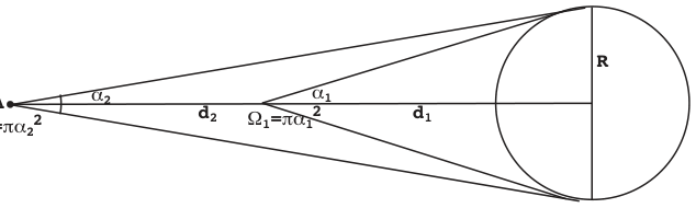
As illustrated in
gure 3.1, the surface brightness of any resolved radiating object
turns out, somewhat surprisingly, to be independent of distance . This is because,
even though the
ux declines with distance, the surface brightness `crowds' this
20 Inferring Stellar Luminosity
d1Ad2α2
Ω2=πα 22α1R
Ω1=πα 12Ω=πα 2α≈ R/d F=L/4πd2I=F/Ω=L/4πd2/πα 2=L/4π2R2=F */πSurface brightness I is
independent of distance d
angular
radiusSolid
angle Flux
Figure 3.1 Distance independence of surface brightness of a radiating sphere,
representing the
ux per solid angle, B=F=
. At greater distance d, the
ux
declines in proportion to 1 =d2; but because this
ux is squeezed into a smaller solid
angle
, which also declines as 1 =d2, the surface brightness Bremains constant,
independent of the distance.
ux into a proportionally smaller solid angle as the distance is increased. The
ratio of
ux per solid angle, or surface brightness, is thus constant.
In particular, if we ignore any absorption from earth's atmosphere, the surface
brightness of the Sun that we see here on earth is actually the same as if we were
standing on the surface of the Sun itself!
Of course, on the surface of the Sun, its radiation will
ll up half the sky {
i.e. 2steradians, instead of the mere 0 :2 deg2= 610�5steradians seen from
earth. The huge
ux from this large, bright solid angle would cause a lot more
than a mere sunburn!1
3.3 Apparent and absolute magnitude and the distance modulus
To summarize, we have now identi
ed 3 distinct kinds of \brightness" { abso-
lute, apparent, and surface { associated respectively with the luminosity (en-
ergy/time),
ux (energy/time/area), and speci
c intensity (
Stellar Magnitudes and Distance Modulus
- Astronomers distinguish between absolute, apparent, and surface brightness, which relate to luminosity, flux, and specific intensity respectively.
- The magnitude system is a logarithmic scale where a difference of 5 magnitudes corresponds to a factor of 100 in relative brightness.
- Apparent magnitude (m) measures how bright a star looks from Earth, while absolute magnitude (M) measures its brightness at a standard distance of 10 parsecs.
- The distance modulus (m - M) is a mathematical relationship used to determine the distance to a star based on its apparent and absolute magnitudes.
- The Sun has an absolute magnitude of approximately +4.8, serving as a baseline for calculating the absolute magnitudes of other stars.
The huge flux from this large, bright solid angle would cause a lot more than a mere sunburn!
Of course, on the surface of the Sun, its radiation will
ll up half the sky {
i.e. 2steradians, instead of the mere 0 :2 deg2= 610�5steradians seen from
earth. The huge
ux from this large, bright solid angle would cause a lot more
than a mere sunburn!1
3.3 Apparent and absolute magnitude and the distance modulus
To summarize, we have now identi
ed 3 distinct kinds of \brightness" { abso-
lute, apparent, and surface { associated respectively with the luminosity (en-
ergy/time),
ux (energy/time/area), and speci
c intensity (
ux emitted into a
given solid angle). Before moving on to examine additional properties of stel-
lar radiation, let us
rst discuss some speci
cs of how astronomers characterize
apparent vs. absolute brightness, namely through the so-called \magnitude" sys-
tem.
This system has some rather awkward conventions, developed through its long
history, dating back to the ancient Greeks. As noted in x1, they ranked the
apparent brightness of stars in 6 bins of magnitude, ranging from m= 1 for
the brightest to m= 6 for the dimmest. Because the human eye is adapted to
1NASA 's recently launched \Parker Solar Probe" will eventually
y within about 9 R
of
the solar surface, or about 1/20 au. So a key challenge has been to provide the shielding
to keep the factor >400 higher solar radiation
ux from frying the spacecraft's instruments.
3.4 Questions and Exercises 21
detect a large dynamic range in brightness, it turns out that our perception of
brightness depends roughly on the logarithm of the
ux.
In our modern calibration this can be related to the Greek magnitude system
by stating that a di
erence of 5 in magnitude represents a factor 100 in the
relative brightness of the compared stars, with the dimmer star having the larger
magnitude . This can be expressed in mathematical form as
m2�m1= 2:5 log(F1=F2): (3.7)
We can further extend this logarithmic magnitude system to characterize the
absolute brightness, a.k.a. luminosity, of a star in terms of an absolute magnitude.
To remove the inherent dependence on distance in the
ux F, and thus in the
apparent magnitude m, the absolute magnitude Mis de
ned as the apparent
magnitude that a star would have if it were placed at a standard distance, chosen
by convention to be d= 10 pc. Since the
ux scales with the inverse-square of
distance,F1=d2, the di
erence between apparent magnitude mand absolute
magnitude Mis given by
m�M= 5 log(d=10 pc); (3.8)
which is known as the distance modulus .
The absolute magnitude of the Sun is M+4.8 (though for simplicity in
calculations, this is often rounded up to 5), and so the scaling for other stars can
be written as
M= 4:8�2:5 log(L=L
): (3.9)
Combining these relations, we see that the apparent magnitude of any star is
given in terms of the luminosity and distance by
m= 4:8�2:5 log(L=L
) + 5 log(d=10 pc): (3.10)
For bright stars, magnitudes can even become negative. For example, the (ap-
parently) brightest star in the night sky, Sirius, has an apparent magnitude
m=�1:42. But with a luminosity of just L23L
, its absolute magnitude is
still positive, M= +1:40. Its distance modulus, m�M=�1:42�1:40 =�2:82,
is negative. Through eqn. (3.8), this implies that its distance, d= 101�2:82=5=
2:7 pc, is lessthan the standard distance of 10 pc used to de
ne absolute mag-
nitude and distance modulus [eqn. (3.8)].
3.4 Questions and Exercises
Quick Question 1: Recalling the relationship between an AU and a parsec from
eqn. (2.6), use eqns. (3.8) and (3.9) to compute the apparent magnitude of the Sun.
What then is the Sun's distance modulus?
Quick Question 2: Suppose two stars have a luminosity ratio L2=L1= 100.
22 Inferring Stellar Luminosity
a. At what distance ratio d2=d1would the stars have the same apparent brightness,
F2=F1?
b. For this distance ratio, what is the di
erence in their apparent magnitude, m2�
m1?
c. What is the di
erence in their absolute magnitude, M2�M1?
Stellar Luminosity and Thermal Radiation
- Mathematical exercises explore the relationships between apparent magnitude, absolute magnitude, and distance modulus for stars and supernovae.
- Stellar brightness is a direct consequence of high surface temperatures, which cause atoms and electrons to collide violently and emit thermal radiation.
- Temperature in astronomy is measured in Kelvins, where absolute zero represents the theoretical limit where all thermal motion ceases.
- Light is defined as electromagnetic radiation consisting of oscillating electric and magnetic fields as described by Maxwell's equations.
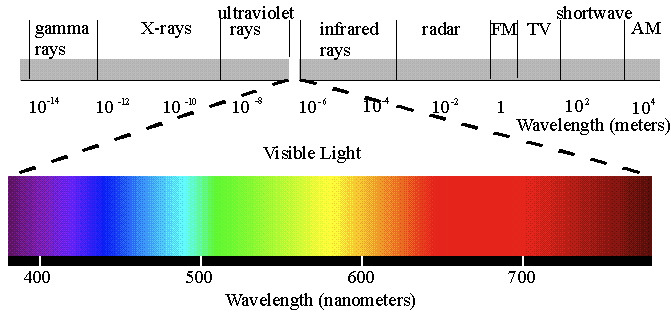
- The electromagnetic spectrum spans from short-wavelength gamma rays to long-wavelength radio waves, with visible light occupying a narrow band between 400 and 750 nm.
- All electromagnetic waves travel at the constant speed of light (c) in a vacuum, maintaining a strict inverse relationship between wavelength and frequency.
The light they emit is called "thermal radiation", and arises from the jostling of the atoms (and particularly the electrons in and around those atoms) by the violent collisions associated with the star's high temperature.
Quick Question 1: Recalling the relationship between an AU and a parsec from
eqn. (2.6), use eqns. (3.8) and (3.9) to compute the apparent magnitude of the Sun.
What then is the Sun's distance modulus?
Quick Question 2: Suppose two stars have a luminosity ratio L2=L1= 100.
22 Inferring Stellar Luminosity
a. At what distance ratio d2=d1would the stars have the same apparent brightness,
F2=F1?
b. For this distance ratio, what is the di
erence in their apparent magnitude, m2�
m1?
c. What is the di
erence in their absolute magnitude, M2�M1?
d. What is the di
erence in their distance modulus?
Quick Question 3: A white-dwarf supernova with peak luminosity L1010L
is
observed to have an apparent magnitude of m= +20 at this peak.
a. What is its Absolute Magnitude M?
b. What is its distance d(in pc and ly). s c. How long ago did this supernova explode
(in Myr)?
(For simplicity of computation, you may take the absolute magnitude of the Sun to
beM
+5.)
4 Inferring Surface Temperature from
a Star's Color and/or Spectrum
Let us next consider why stars shine with such extreme brightness. Over the
long-term (i.e., millions of years), the enormous energy emitted comes from the
energy generated (by nuclear fusion) in the stellar core, as discussed further in x18
below. But the more immediate reason stars shine is more direct, namely because
their surfaces are so very hot. The light they emit is called \thermal radiation",
and arises from the jostling of the atoms (and particularly the electrons in and
around those atoms) by the violent collisions associated with the star's high
temperature1.
Figure 4.1 The Electromagnetic Spectrum.
1In astronomy, temperature is measured in a degree unit called a Kelvin , abbreviated K,
and de
ned relative to the centigrade or \Celsius" scale C such that K=C+ 273. A
temperature of T= 0Kis called \absolute zero", and represents the ideal limit that all
thermal motion is completely stopped. To convert from our US use of the Fahrenheit scale
F, we
rst just convert to centigrade using C= (5=9)(F�32), and then add 273 to get the
temperature in K.
24 Inferring Surface Temperature from a Star's Color and/or Spectrum
4.1 The wave nature of light
To lay the groundwork for a general understanding of the key physical laws
governing such thermal radiation and how it depends on temperature, we have
to review what is understood about the basic nature of light, and the processes
by which it is emitted and absorbed.
The 19th century physicist James Clerk Maxwell developed a set of 4 equations
(Maxwell's equations) that showed how variations in Electric and Magnetic
elds
could lead to oscillating wave solutions, which he indeed indentifed with light,
or more generally Electro-Magnetic (EM) radiation . The wavelengths of these
EM waves are key to their properties. As illustrated in
gure 4.1, visible light
corresponds to wavelengths ranging from 400 nm (violet) to 750 nm
(red), but the full spectrum extends much further, including Ultra-Violet (UV),
X-rays, and gamma rays at shorter wavelengths, and InfraRed (IR), microwaves,
and radio waves at longer wavelengths. White light is made up of a broad mix
of visible light ranging from Red through Green to Blue (RGB).
In a vacuum, all these EM waves travel at the same speed , namely the speed
of light, customarily denoted as c, with a value c3105km/s = 3108m/s
= 31010cm/s. The wave period is the time it takes for a complete wavelength
to pass a
xed point at this speed, and so is given by P==c. We can thus
see that the sequence of wave crests passes by at a frequency of once per period,
= 1=P, implying a simple relationship between light's wavelength , frequency
, and speed c,
P==c: (4.1)
4.2 Light quanta and the Black-Body emission spectrum
The wave nature of light has been con
rmed by a wide range experiments. How-
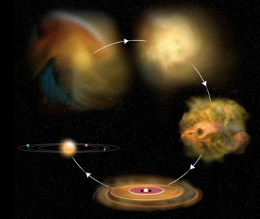
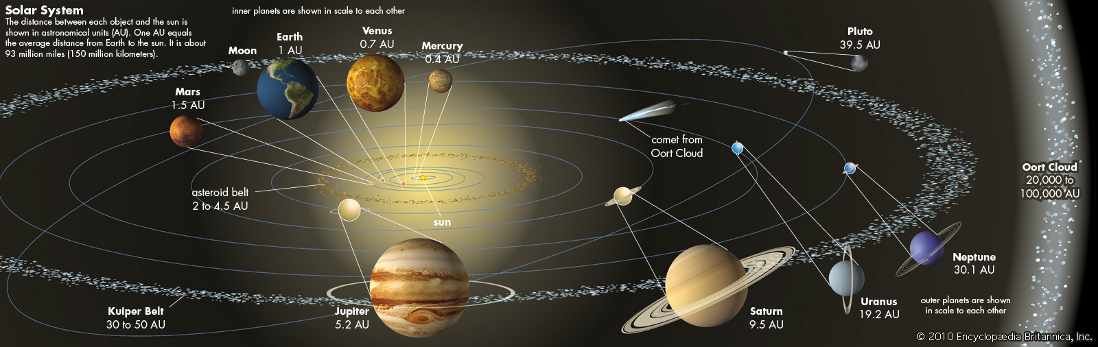
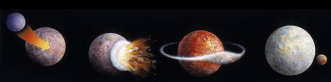
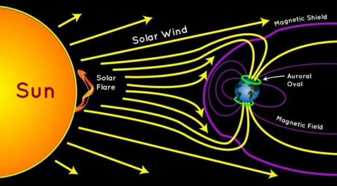
Light Quanta and Black-Body Radiation
- Light exhibits a dual nature, behaving as both a wave with a specific frequency and wavelength and as discrete bundles of energy called photons.
- The energy of a photon is directly proportional to its frequency, a discovery by Planck and Einstein that established the quantization of energy.
- A Black Body is an idealized material in thermodynamic equilibrium that emits a Spectral Energy Distribution (SED) dependent solely on its temperature.
- The Planck function describes how the intensity or surface brightness of this radiation is distributed across different wavelengths or frequencies.
- Wien's Displacement Law shows that the peak wavelength of emission shifts to shorter, bluer wavelengths as the temperature of the object increases.
- By measuring the peak wavelength of a star's light, astronomers can calculate its surface temperature, such as the Sun's 5800K temperature based on its 500 nm peak.
Each photon carries a discrete, indivisible 'quantum' of energy that depends on the wave frequency.
of light, customarily denoted as c, with a value c3105km/s = 3108m/s
= 31010cm/s. The wave period is the time it takes for a complete wavelength
to pass a
xed point at this speed, and so is given by P==c. We can thus
see that the sequence of wave crests passes by at a frequency of once per period,
= 1=P, implying a simple relationship between light's wavelength , frequency
, and speed c,
P==c: (4.1)
4.2 Light quanta and the Black-Body emission spectrum
The wave nature of light has been con
rmed by a wide range experiments. How-
ever, at the beginning of the 20th century, work by Einstein, Planck, and others
led to the realization that light waves are also quantized into discrete wave \bun-
dles" called photons . Each photon carries a discrete, indivisible \quantum" of
energy that depends on the wave frequency as
E=h; (4.2)
wherehisPlanck's constant , with value h6:610�27erg s = 6:610�34
Joule s.
This quantization of light (and indeed of all energy) has profound and wide-
ranging consequences, most notably in the current context for how thermally
emitted radiation is distributed in wavelength or frequency. This is known as the
\Spectral Energy Distribution" (SED). For a so-called Black Body { meaning
4.2 Light quanta and the Black-Body emission spectrum 25
5500K
5000K
4000K
3500K4500K
0 500 1000 1500 200005.0×1061.0×1071.5×1072.0×107
λ(nm)Bλ(erg/s/cm2/nm)
Figure 4.2 The Planck Black-Body Spectral Energy Distribution (SED) vs.
wavelength , plotted for various temperatures T.
idealized material that is readily able to absorb and emit radiation of all wave-
lengths {, Planck showed that as thermal motions of the material approach a
Thermodynamic Equilibrium (TE) in the exchange of energy between radiation
and matter, the SED can be described by a function that depends onlyon the gas
temperature T(and not, e.g., on the density, pressure, or chemical composition).
In terms of the wave frequency , this Planck Black-Body function takes the
form
B(T) =2h3=c2
eh=kT�1; (4.3)
wherekis Boltzmann's constant, with value k= 1:3810�16erg/K = 1:38
10�23Joule/K. For an interval of frequency between and+d, the quantity
Bdgives the emitted energy per unit time per unit area per unit solid an-
gle. This means the Planck Black-Body function is fundamentally a measure of
intensity orsurface brightness , withBrepresenting the distribution of surface
brightness over frequency , having CGS units erg/cm2/s/ster/Hz (and MKS
units W/m2/ster/Hz).
Sometimes it is convenient to instead de
ne this Planck distribution in terms of
the brightness distribution in a wavelength interval between and+d,Bd.
Requiring that this equals Bd, and noting that =c=impliesjd=dj=c=2,
we can use eqn. (4.3) to obtain
B(T) =2hc2=5
ehc=kT�1: (4.4)
26 Inferring Surface Temperature from a Star's Color and/or Spectrum
4.3 Inverse-temperature dependence of wavelength for peak
ux
Figure 4.2 plots the variation of Bvs. wavelength for various temperatures
T. Note that for higher temperature, the level of Bis higher at allwavelengths,
with greatest increases near the peak level.
Moreover, the location of this peak shifts to shorter wavelength with higher
temperature. We can determine this peak wavelength maxby solving the equa-
tiondB
d
=max0: (4.5)
Leaving the details as an exercise, the result is
max=2:9106nm K
T=290 nm
T=10;000K500 nm
T=T
; (4.6)
which is known as Wien's displacement law .
For example, the last equality uses the fact that the observed wavelength peak
in the Sun's spectrum is max;
500 nm, very near the the middle of the visible
spectrum.2We can solve for a Black-Body-peak estimate for the Sun's surface
temperature
T
=2:9106nm K
500 nm= 5800K: (4.7)
By similarly measuring the peak wavelength maxin other stars, we can likewise
derive an estimate of their surface temperature by
T=T
max;
max5800K500 nm
max: (4.8)
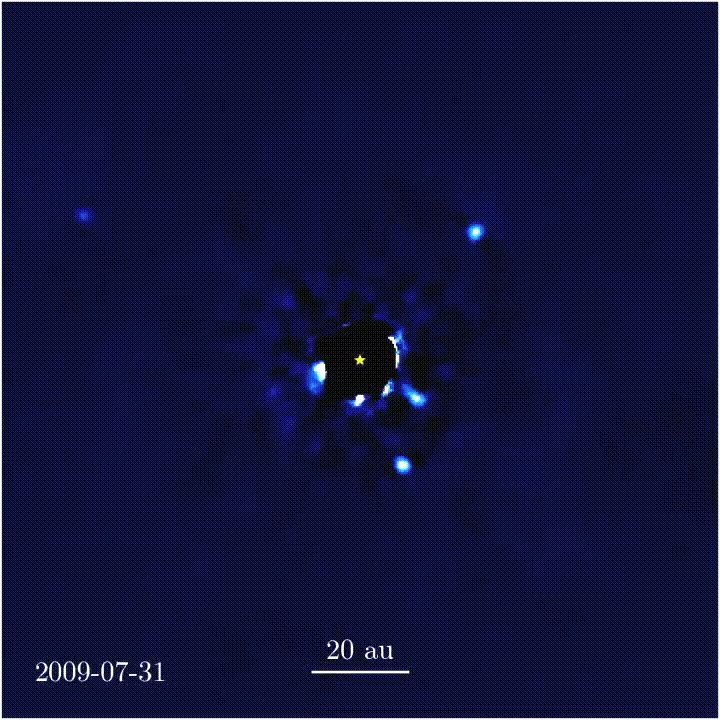
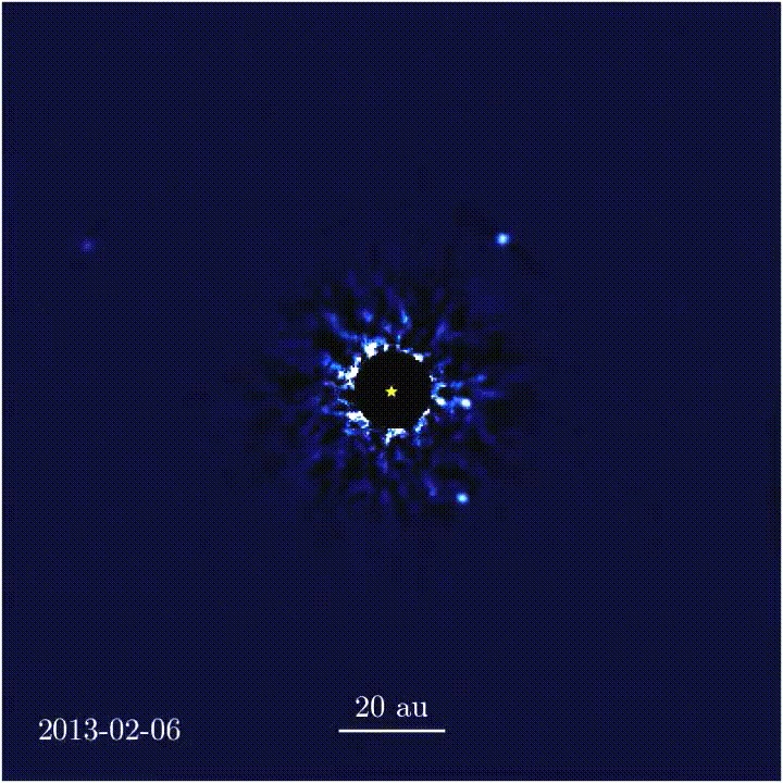
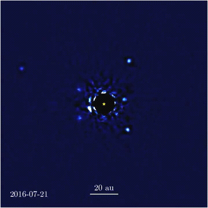
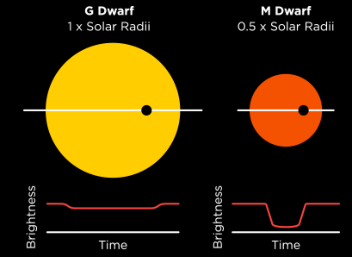
Measuring Stellar Temperatures
- Wien's displacement law provides a direct mathematical relationship between a star's peak wavelength and its surface temperature.
- The Sun's peak wavelength of 500 nm corresponds to a surface temperature of approximately 5800 K, placing its brightest emission in the visible spectrum.
- Human vision likely evolved to be most sensitive to the specific wavelengths where solar illumination is at its peak intensity.
- In practice, astronomers use photometric color systems like the Johnson UBV filters because measuring a full spectral energy distribution is difficult and time-consuming.
- The 'color index' (such as B-V) serves as a distance-independent diagnostic for temperature, where negative values indicate hotter, bluer stars.
This is not entirely coincidental, since our eyes evolved to use the wavelengths of light for which the solar illumination is brightest.
T=10;000K500 nm
T=T
; (4.6)
which is known as Wien's displacement law .
For example, the last equality uses the fact that the observed wavelength peak
in the Sun's spectrum is max;
500 nm, very near the the middle of the visible
spectrum.2We can solve for a Black-Body-peak estimate for the Sun's surface
temperature
T
=2:9106nm K
500 nm= 5800K: (4.7)
By similarly measuring the peak wavelength maxin other stars, we can likewise
derive an estimate of their surface temperature by
T=T
max;
max5800K500 nm
max: (4.8)
4.4 Inferring stellar temperatures from photometric colors
In practice, this is not quite the approach to estimating a star's temperature
that is most commonly used in astronomy, in part because with real SEDs, it
is relatively dicult to identify accurately the peak wavelength. Moreover in
surveying a large number of stars, it requires a lot more e
ort (and telescope
time) to measure the full SED, especially for relatively faint stars. A simpler,
more common method is just to measure the stellar color .
But rather than using the Red, Green, and Blue (RGB) colors we perceive
with our eyes, astronomers typically de
ne a set of standard colors that extend
to wavebands beyond just the visible spectrum. The most common example is
the Johnson 3-color UBV (Ulraviolet, Blue, Visible) system. The left panel of
2This is not entirely coincidental, since our eyes evolved to use the wavelengths of light for
which the solar illumination is brightest.
4.5 Questions and Exercises 27
U
B
V
Eye
200 300 400 500 600 700 800 9000.00.20.40.60.81.0
Wavelength(nm)Sensitivity
⊙ ⊙
-0.5 0.0 0.5 1.0 1.5 2.0500010 00015 00020 000
Color Index B-VSurface Temperture(K)
Figure 4.3 Left: Comparison of the spectral sensitivity of the human eye with those
the UBV
lters in the Johnson photometric color system. Right: Temperature
dependence of the B-V color for a Black-Body emitted spectrum. The circle dot
marks the solar values T
5800 K and ( B�V)
0:656.
gure 4.3 compares the wavelength sensitivity of such UBV
lters to that of the
human eye. By passing the star's light through a standard set of
lters designed
to only let through light for the de
ned color waveband, the observed apparent
brightness in each
lter can be used to de
ne a set of color magnitudes, e.g.
mU;mB, andmV.
The standard shorthand is simply to denote these color magnitudes just by
the capital letter alone, viz. U, B, and V. The di
erence between two color
magnitudes, e.g. B�VmB�mV, is independent of the stellar distance,
but provides a direct diagnostic of the stellar temperature, sometimes called the
\color temperature".
Because a larger magnitude corresponds to a lower brightness, stars with a
positive B-V actually are less bright in the blue than in the visible, implying
a relatively lowtemperature. On the other hand, a negative B-V means blue
is brighter, implying a high temperature. The right panel of
gure 4.3 shows
how the temperature of a Black-Body varies with the B-V color of the emitted
Black-Body spectrum.
4.5 Questions and Exercises
Quick Question 1: Two photons have wavelength ratio 2=1= 2.
a. What is the ratio of their period P2=P1?
b. What is the ratio of their frequency 2=1?
c. What is the ratio of their energy E2=E1?
Quick Question 2:
28 Inferring Surface Temperature from a Star's Color and/or Spectrum
a. Estimate the temperature of stars with max=100, 300, 1000, and 3000 nm. (To
simplify the numerics, you may take T
6000 K.)
b. Conversely, estimate the peak wavelengths maxof stars with T=2000, 10,000,
and 60, 000 K.
c. What parts of the EM spectrum (i.e. UV, visible, IR) do each of these lie in?
Quick Question 3:
a. Assuming the Earth has an average temperature equal to that of typical spring
day, i.e. 50F, compute the peak wavelength of Earth's Black-Body radiation.
b. What part of the EM spectrum does this lie in?
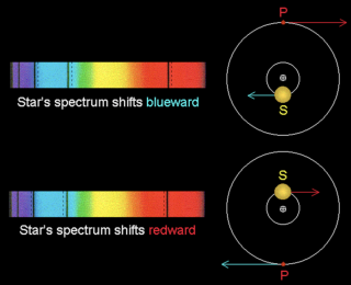
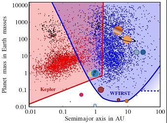
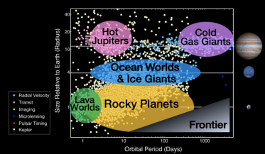
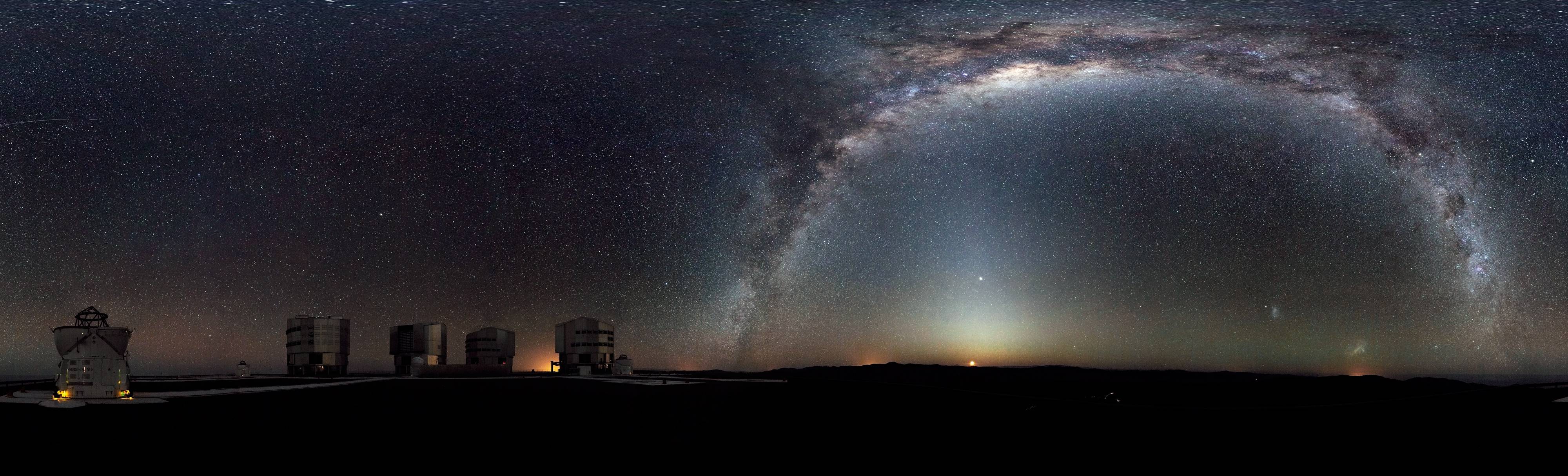
Stellar Radius and Stefan-Boltzmann Law
- The Stefan-Boltzmann law establishes that the total energy emitted by a blackbody increases sharply with the fourth power of its temperature.
- Stellar luminosity is determined by the combination of a star's surface temperature and its total surface area.
- By measuring a star's flux and temperature, astronomers can mathematically derive its physical radius.
- The relationship between luminosity, temperature, and radius is often simplified by scaling values against those of the Sun.
- While blackbody radiation provides a foundational model, real stellar spectra are complicated by discrete absorption lines.
The Stefan-Boltzmann law is one of the linchpins of stellar astronomy.
a. Estimate the temperature of stars with max=100, 300, 1000, and 3000 nm. (To
simplify the numerics, you may take T
6000 K.)
b. Conversely, estimate the peak wavelengths maxof stars with T=2000, 10,000,
and 60, 000 K.
c. What parts of the EM spectrum (i.e. UV, visible, IR) do each of these lie in?
Quick Question 3:
a. Assuming the Earth has an average temperature equal to that of typical spring
day, i.e. 50F, compute the peak wavelength of Earth's Black-Body radiation.
b. What part of the EM spectrum does this lie in?
Exercise 1: UsingBd=Bdand the relationship between frequency and wave-
length, derive eqn. (4.4) from eqn. (4.3).
Exercise 2: Derive eqn. (4.6) from eqn. (4.4) using the de
nition (4.5).
5 Inferring Stellar Radius from
Luminosity and Temperature
We see from
gure 4.2 that, in addition to a shift toward shorter peak wavelength
max, a higher temperature also increases the overall brightness of blackbody
emission at allwavelengths. This suggests that the total energy emitted over all
wavelengths should increase quite sharply with temperature. Leaving the details
as an exercise for the reader, let us quantify this expectation by carrying out
the necessary spectral integrals to obtain the temperature dependence of the
Bolometric intensity of a blackbody
B(T)Z1
0B(T)d=Z1
0B(T)d=sbT4
; (5.1)
withsb= 25k4=(15h3c2) known as the Stefan-Boltzmann constant, with nu-
merical value sb= 5:6710�5erg/cm2/s/K4= 5:6710�8J/m2/s/K4.
If we spatially resolve a pure blackbody with surface temperature T, then
B(T) represents the Bolometric surface brightness we would observe from each
part of the visible surface.
5.1 Stefan-Boltzmann law for surface
ux from a blackbody
Combining eqns. (3.6) and (5.1), we see that the radiative
uxat the surface
radiusRof a blackbody is given by
FF(R) =B(T) =sbT4; (5.2)
which is known as the Stefan-Boltzman law .
The Stefan-Boltzmann law is one of the linchpins of stellar astronomy. If we
now relate the surface
ux to the stellar luminosity Lover the surface area 4 R2,
then applying this to the Stefan-Boltzmann law gives
L=sbT44R2; (5.3)
which is often more convenient to scale by associated solar values,
L
L
=T
T
4R
R
2
: (5.4)
30 Inferring Stellar Radius from Luminosity and Temperature
We can also use eqn. (5.3) to solve for the stellar radius,
R=r
L
4sbT4=s
F(d)
sbT4d; (5.5)
where the latter equation uses the inverse-square-law to relate the stellar radius
to the
ux F(d) and distance d, along with the surface temperature T.
For a star with a known distance d, e.g. by a measured parallax, measurement
of apparent magnitude gives the
ux F(d), while measurement of the peak wave-
lengthmaxor color (e.g. B-V) provides an estimate of the temperature T(see
gure 4.3). Applying these in eqn. (5.5), we can thus obtain an estimate of the
stellar radius R.
5.2 Questions and Exercises
Quick Question 1: Compute the luminosity L(in units of the solar luminosity L
),
absolute magnitude M, and peak wavelength max(in nm) for stars with (a) T=T
;
R= 10R
, (b)T= 10T
;R=R
, and (c)T= 10T
;R= 10R
. If these stars all
have a parallax of p= 0:001 arcsec, compute their associated apparent magnitudes m.
Quick Question 2: Suppose a star has a parallax p= 0:01 arcsec, peak wavelength
max= 250 nm, and apparent magnitude m= +5 . About what is its:
a. Distance d(in pc)?
b. Distance modulus m�M?
c. Absolute magntidue M?
d. Luminosity L(inL
)?
e. Surface temperature T(inT
)?
f. RadiusR(inR
)?
g. Angular radius
(in radian and arcsec)?
h. Solid angle
(in steradian and arcsec2)?
i. Surface brightness relative to that of the Sun, B=B
?
6 Absorption Lines in Stellar Spectra
Figure 6.1 The Sun's spectrum, showing the complex pattern of absorption lines at
discrete wavelength or colors. [NOAO/AURA/NSF]
In reality stars are not perfect blackbodies, and so their emitted spectra don't
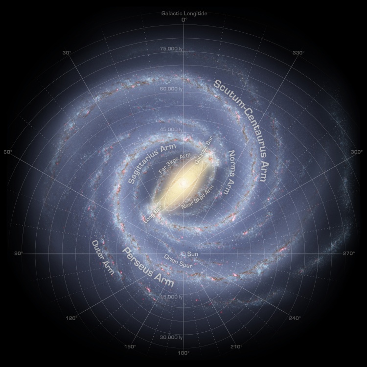
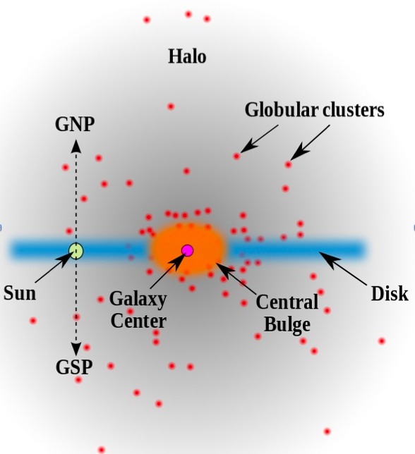
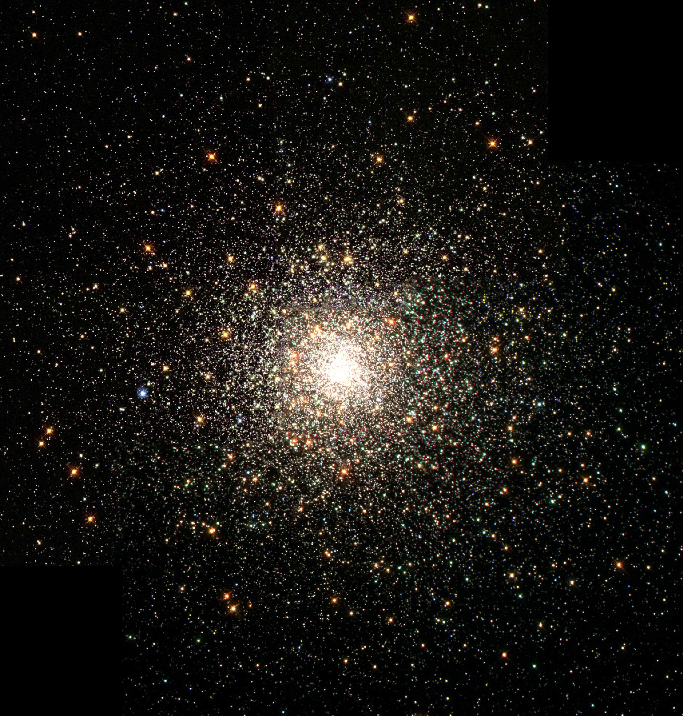
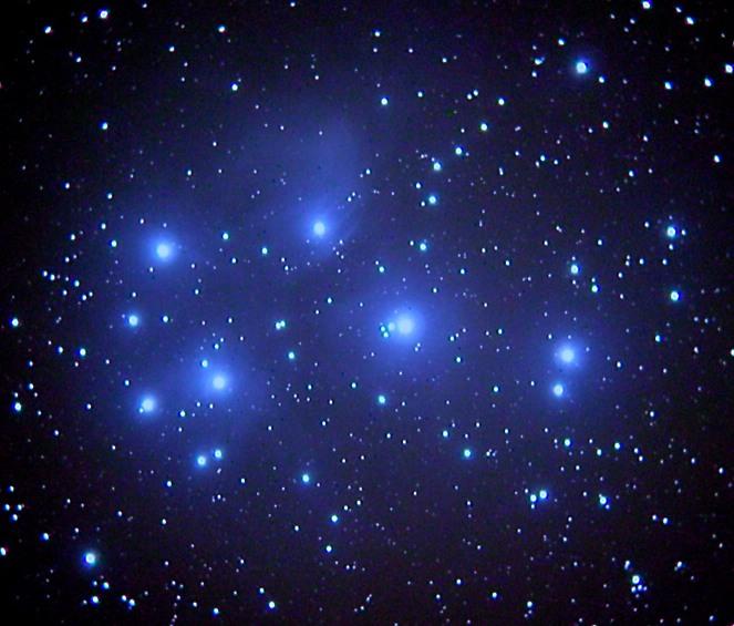
Stellar Absorption Line Spectra
- Stars are not perfect blackbodies because their spectra contain detailed signatures of elemental composition rather than just temperature.
- The interior heat of a star diffuses outward through a temperature gradient, interacting with atoms and ions in the cooler surface layers.
- Atomic energy levels are quantized like steps in a staircase, meaning atoms only efficiently absorb photons that match specific energy differences.
- The resulting missing light appears as a complex series of dark absorption lines when a star's spectrum is spread out by a prism.
- These absorption lines act as a unique fingerprint or barcode that identifies the specific elements and ionization stages present in a star's atmosphere.
- Laboratory measurements of known elements allow scientists to decode these stellar fingerprints to determine chemical composition.
As such the associated wavelengths of the absorption lines in a star's spectrum provide a direct 'fingerprint' — perhaps even more akin to a supermarket bar code — for the presence of that element in the star's atmosphere.
max= 250 nm, and apparent magnitude m= +5 . About what is its:
a. Distance d(in pc)?
b. Distance modulus m�M?
c. Absolute magntidue M?
d. Luminosity L(inL
)?
e. Surface temperature T(inT
)?
f. RadiusR(inR
)?
g. Angular radius
(in radian and arcsec)?
h. Solid angle
(in steradian and arcsec2)?
i. Surface brightness relative to that of the Sun, B=B
?
6 Absorption Lines in Stellar Spectra
Figure 6.1 The Sun's spectrum, showing the complex pattern of absorption lines at
discrete wavelength or colors. [NOAO/AURA/NSF]
In reality stars are not perfect blackbodies, and so their emitted spectra don't
just depend on temperature, but contain detailed signatures of key physical
properties like elemental composition. The energy we see emitted from a stellar
surface is generated in the very hot interior and then di
uses outward, following
the strong temperature decline to the surface. The atoms and ions that absorb
and emit the light don't do so with perfect eciency at all wavelengths, which
is what is meant by the \black" in \blackbody". We experience this all the
time in our everyday world, which shows that di
erent objects have distinct
\color", meaning they absorb certain wavebands of light, and re
ect others. For
example, a green leaf re
ects some of the \green" parts of the visible spectrum
{ with wavelengths near 5100 A{ and absorbs most of the rest.
For atoms in a gas, the ability to absorb, scatter and emit light can likewise
32 Absorption Lines in Stellar Spectra
Figure 6.2 Illustration of principals for producing an emission vs. an absorption line
spectrum. The left panel shows that an incandescent light passed through a prism
generally produces a featureless continuum spectrum, but a cold gas placed in front of
this yields an absorption line spectrum. That same gas when heated and seen on its
own against a dark background produces the same pattern of lines, but now in
emission instead of absorption. The right panel shows heuristically how the relatively
cool gas in the surface layers of a star leads to an absorption line spectrum from the
star.
depend on the wavelength, sometimes quite sharply. Just as the energy of light is
quantized into discrete bundles called photons, the energy of electrons orbiting an
atomic nucleus have discrete levels, much like the steps in a staircase. Absorption
or scattering by the atom is thus much more ecient for those select few photons
with an energy that closely matches the energy di
erence between two of these
atomic energy levels.
The evidence for this is quite apparent if we examine carefully the actual spec-
trum emitted by any star. Although the overall \Spectral Energy Distribution"
(SED) discussed above often roughly
ts a Planck Black-Body function, careful
inspection shows that light is missing or reduced at a number of discrete wave-
lengths or colors. As illustrated in
gure 6.1 for the Sun, when the color spectrum
of light is spread out, for example by a prism or di
raction grating, this missing
light appears as a complex series of relatively dark \absorption lines".
Figure 6.2 illustrates how the absorption by relatively cool, low-density atoms
in the upper layers of the Sun or a star's atmosphere can impart this pattern of
absorption lines on the continuum, nearly Black-Body spectrum emitted by the
denser, hotter layers.
A key point here is that the discrete energies levels associated with atoms
of di
erent elements (or, as discussed below, di
erent \ionization stages" of a
given element) are quite distinct. As such the associated wavelengths of the
absorption lines in a star's spectrum provide a direct \
ngerprint" { perhaps
even more akin to a supermarket bar code { for the presence of that element in
the star's atmosphere. The code \key" can come from laboratory measurement
of the line-spectrum from known samples of atoms and ions, or, as discussed in
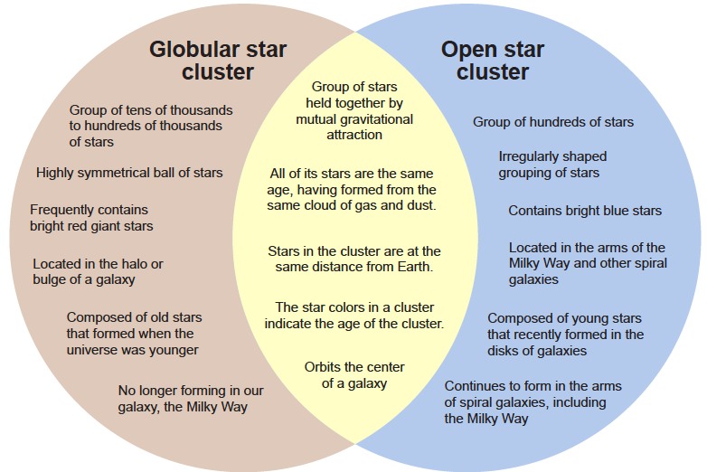
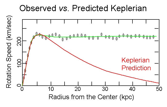
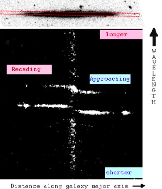
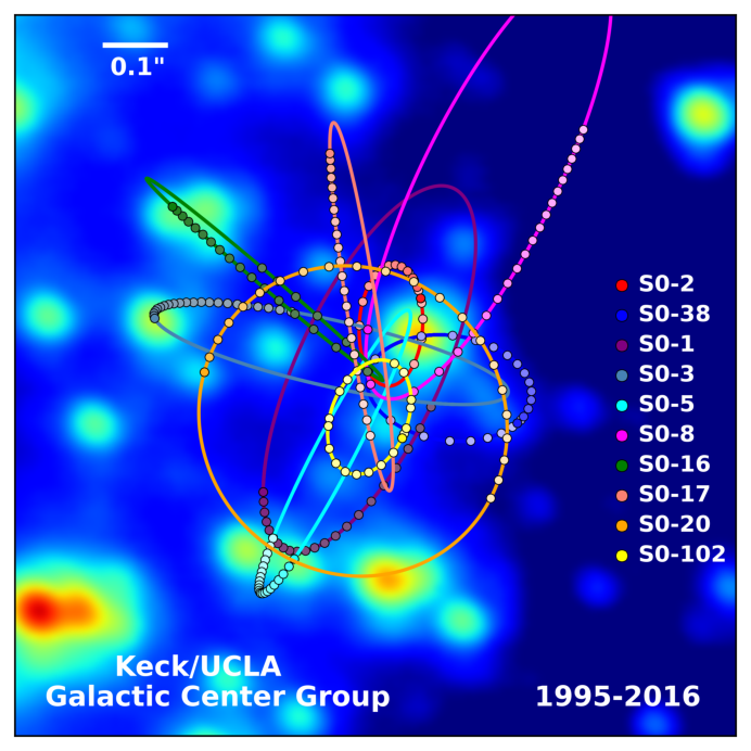
Stellar Fingerprints and Composition
- Absorption lines in a star's spectrum act as a unique 'barcode' or fingerprint for identifying specific chemical elements.
- The Sun and most stars are composed almost entirely of hydrogen (90.9%) and helium (8.9%), with all other elements making up only 0.2% of the total atoms.
- In astronomy, all elements heavier than hydrogen and helium are collectively referred to as 'metals,' accounting for a mass fraction of about 2%.
- Earth's composition mirrors the Sun's heavier elements, but our planet lost its lighter gases like hydrogen and helium due to its weaker gravity.
- Stellar spectral types (OBAFGKM) are determined by surface temperature, which dictates the ionization stages of the elements present.
The associated wavelengths of the absorption lines in a star's spectrum provide a direct 'fingerprint'—perhaps even more akin to a supermarket bar code—for the presence of that element in the star's atmosphere.
denser, hotter layers.
A key point here is that the discrete energies levels associated with atoms
of di
erent elements (or, as discussed below, di
erent \ionization stages" of a
given element) are quite distinct. As such the associated wavelengths of the
absorption lines in a star's spectrum provide a direct \
ngerprint" { perhaps
even more akin to a supermarket bar code { for the presence of that element in
the star's atmosphere. The code \key" can come from laboratory measurement
of the line-spectrum from known samples of atoms and ions, or, as discussed in
xA.1, from theoretical models of the atomic energy levels using modern principles
of quantum physics.
6.1 Elemental composition of the Sun and stars 33
H H
He He
Li Li
Be BeB BC C
N NO O
F FNe Ne
Na NaMg Mg
Al AlSi Si
P PS S
Cl ClAr Ar
K KCa Ca
Sc ScTi Ti
V VCr CrMn MnFe Fe
Co CoNi Ni
Cu CuZn Zn
Ga GaGe Ge
As AsSe Se
Br BrKr Kr
Rb RbSr Sr
Y YZr Zr
Nb NbMo MoRu Ru
Rh RhPd Pd
Ag AgCd Cd
In InSn Sn
Sb SbTe Te
I IXe Xe
Cs CsBa Ba
La LaCe Ce
Pr PrNd NdSm Sm
Eu EuGd Gd
Tb TbDy Dy
Ho HoEr Er
Tm TmYb Yb
Lu LuHf Hf
Ta TaW WRe ReOs OsIr IrPt Pt
Au AuHg HgTl TlPb Pb
Bi BiTh ThU U
0 20 40 60 8010-1110-810-50.01
Atomic NumberRelative Abundance by Number
Figure 6.3 Number fractions of elements, plotted on a log scale vs. atomic number,
with data points labeled by the symbols for each element.
6.1 Elemental composition of the Sun and stars
With proper physical modeling, the relative strengths of the absorption lines
can even provide a quantitative measure of the relative abundance of the various
elements. A key result is that the composition of the Sun, which is typical of
most all stars, is dominated by just the two simplest elements, namely Hydrogen
(H) and Helium (He) { which make up respectively 90.9% and 8.9% of the atoms,
with all the other only about 0.2%. Figure 6.3 gives a log plot of these number
fractions vs. atomic number.
The corresponding mass fractions are X0:72 andY0:26 for Hydrogen
and Helium. All the remaining elements of the periodic table { commonly referred
to in astronomy as \metals" { make up just the
nal two percent of the mass.,
denoted as a \metalicity" Z0:02. Of these, the most abundant are Oxygen,
Carbon, and Iron, with respective mass fractions of 0.009, 0.003, and 0.001.
Like all the planets in our solar system, the Earth formed out of the same
material that makes up the Sun ( x23). But its relatively weak gravity has allowed
a lot of the light elements like Hydrogen and Helium to escape into space, leaving
behind the heavier elements that make up our world, and us ( x24). Indeed, once
the H and He are removed, the relative abundances of all these s elements are
roughly the same on the Earth as in the Sun!
34 Absorption Lines in Stellar Spectra
6.2 Stellar spectral type: ionization abundances as temperature
diagnostic
Figure 6.4 Stellar spectra for the full range of spectral types OBAFGKM,
corresponding to a range in stellar surface temperature from hot to cool.
[NOAO/AURA/NSF]
Another key factor in the observed stellar spectra is that the atomic elements
present are generally not electrically neutral, but typically have had one or more
electrons stripped { ionized| by thermal collisions with characteristic energies
set by the temperature. As such, the observed degree of ionization depends on
the temperature near the visible stellar surface. Figure 6.4 compares the spec-
tra of stars of di
erent surface temperature, showing that this leads to gradual
changes and shifts in the detailed pattern of absorption lines from the various
ionizations stages of the various elements. The letters \OBAFGKM" represent
various categories, known as spectral class or \spectral type", assigned to stars
with di
erent spectral patterns. It turns out that type O is the hottest, with tem-
peratures about 50,000 K, while M is the coolest1with temperatures of about
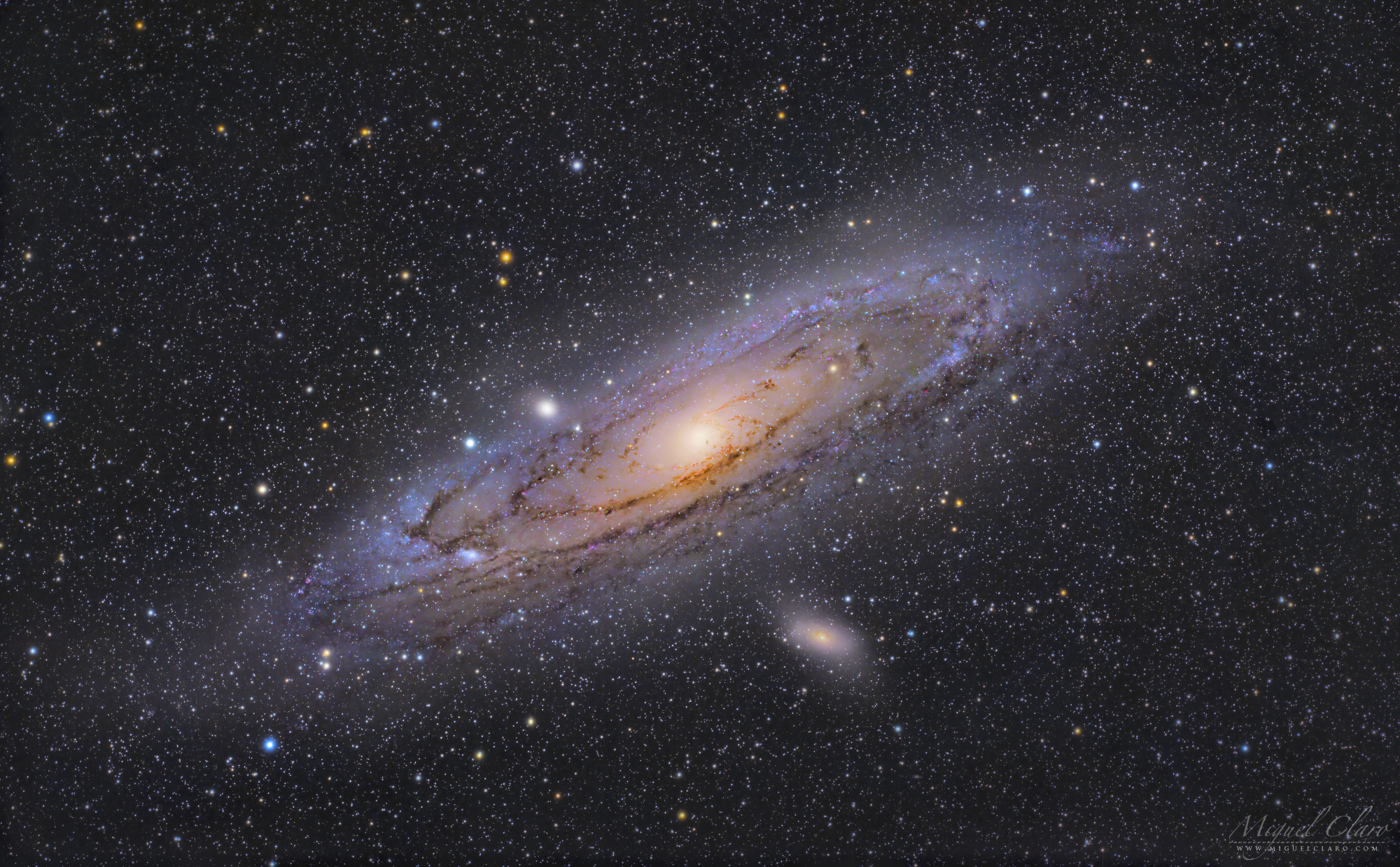
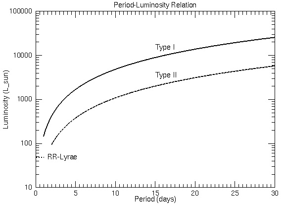
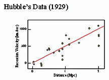
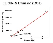
Spectral Classification and H-R Diagrams
- Stars are categorized into spectral types (OBAFGKM) based on surface temperature, ranging from 50,000 K to 3,500 K.
- Luminosity classes, denoted by Roman numerals I through V, distinguish between massive supergiants and smaller dwarf stars.
- The Sun is classified as a G2V star, representing an average temperature and a dwarf-scale luminosity.
- Absorption lines in stellar spectra serve as markers for measuring the Doppler effect and identifying chemical composition.
- The Hertzsprung-Russell (H-R) diagram is a fundamental tool that relates a star's luminosity to its surface temperature.
- Brown dwarfs (classes LTY) represent a bridge between the coolest stars and gas giant planets like Jupiter.
In summary, the appearance of absorption lines in stellar spectra provides a real treasure trove of clues to the physical properties of stars.
the temperature near the visible stellar surface. Figure 6.4 compares the spec-
tra of stars of di
erent surface temperature, showing that this leads to gradual
changes and shifts in the detailed pattern of absorption lines from the various
ionizations stages of the various elements. The letters \OBAFGKM" represent
various categories, known as spectral class or \spectral type", assigned to stars
with di
erent spectral patterns. It turns out that type O is the hottest, with tem-
peratures about 50,000 K, while M is the coolest1with temperatures of about
3500 K. The sequence is often remembered through the mnemonic2\Oh, Be A
Fine Gal/Guy Kiss Me". In keeping with its status as a kind of average star,
the Sun has spectral type G, just a bit cooler than type F in the middle of the
sequence.
In addition to the spectral classes OBAFGKM that depend on surface temper-
atureT, spectra can also be organized in terms of luminosity classes, convention-
1In recent years, it has become possible to detect even cooler \Brown dwarf" stars, with
spectral classes LTY, extending down to temperatures as low as 1000 K. Brown dwarf
stars have too low a mass ( <0:08M
) to force hydrogen fusion in their interior (see
x16.3). They represent a link to gas giant planets like Jupiter (for which MJ0:001M
).
2A student in one of my exams once o
ered an alternative mnemonic: \Oh Boy, Another
F's Gonna Kill Me".
6.3 Hertzsprung-Russell (H-R) diagram 35
ally denoted though Roman numerals I for the biggest, brightest \supergiant"
stars, to V for smaller, dimmer \dwarf" stars; in between, there are luminosity
classes II (bright giants), III (giants), and IV (sub-giants).
In this two-parameter scheme, the Sun is classi
ed as a G2V star.
Finally, in addition to giving information on the temperature, chemical compo-
sition, and other conditions of a star's atmosphere, these absorption lines provide
convenient \markers" in the star's spectrum. As discussed in x9.2, this makes
it possible to track small changes in the wavelength of lines that arise from the
so-called Doppler e
ect as a star moves toward or away from us.
In summary, the appearance of absorption lines in stellar spectra provides a
real treasure trove of clues to the physical properties of stars.
Figure 6.5 Left: Hertzsprung-Russel (H-R) diagram relating star's absolute magnitude
(or log luminosity ) vs. surface temperature, as characterized by the spectral type or
color, with hotter bluer stars on the left, and cooler redder stars on the right. The
main sequence (MS) represents stars burning Hydrogen into Helium in their core,
whereas the giants are supergiants are stars that have evolved away from the MS
after exhausting Hydrogen in their cores. The White Dwarf stars are dying remnants
of solar-type stars. Right: Observed H-R diagram for stars in the solar neighborhood.
The points include 22,000 stars from the Hipparcos Catalogue together with 1000
low-luminosity stars (red and white dwarfs) from the Gliese Catalogue of Nearby
Stars.
6.3 Hertzsprung-Russell (H-R) diagram
A key diagnostic of stellar populations comes from the Hertzsprung-Russel (H-
R) diagram, illustrated by the left panel of
gure 6.5. Observationally, it relates
(absolute) magnitude (or luminosity class) on the y-axis, to color or spectral
36 Absorption Lines in Stellar Spectra
type on the x-axis; physically, it relates luminosity to temperature. For stars in
the solar neighborhood with parallaxes measured by the Hipparchus astrometry
satellite, one can readily use the associated distance to convert observed apparent
magnitudes to absolute magnitudes and luminosities. The right panel of
gure 6.5
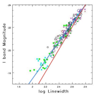
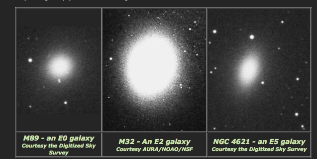
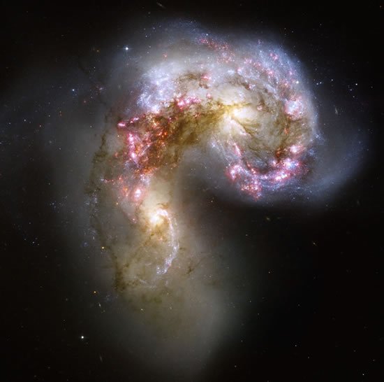
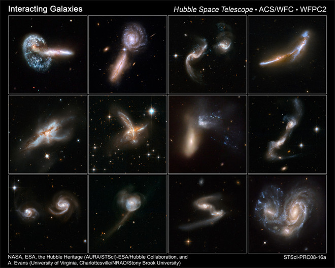
The Hertzsprung-Russell Diagram
- The H-R diagram relates a star's absolute magnitude or luminosity to its color, spectral type, or temperature.
- The main sequence represents the longest phase of a star's life, characterized by stable hydrogen burning in the core.
- Giant and supergiant stars represent later evolutionary stages where stars burn heavier elements or hydrogen in shells.
- White dwarfs are the final, cooling remnants of low-mass stars like the Sun, positioned below the main sequence.
- The H-R diagram serves as a vital link between observable surface light and the physical evolution of a star's interior.
- Mass and age are identified as the two primary parameters that differentiate stars across the diagram's various regions.
The reason there are so many stars in this main-sequence band is that it represents the long-lived phase when stars are stably burning Hydrogen into Helium in their cores.
R) diagram, illustrated by the left panel of
gure 6.5. Observationally, it relates
(absolute) magnitude (or luminosity class) on the y-axis, to color or spectral
36 Absorption Lines in Stellar Spectra
type on the x-axis; physically, it relates luminosity to temperature. For stars in
the solar neighborhood with parallaxes measured by the Hipparchus astrometry
satellite, one can readily use the associated distance to convert observed apparent
magnitudes to absolute magnitudes and luminosities. The right panel of
gure 6.5
shows the H-R diagram for these stars, plotting their known luminosities vs. their
colors or spectral types, with the horizontal lines showing the luminosity classes3.
The extended band of stars running from the upper left to lower right is known
as the main sequence , representing \dwarf" stars of luminosity class V. The
reason there are so many stars in this main-sequence band is that it represents
the long-lived phase when stars are stably burning Hydrogen into Helium in their
cores (x18).
The medium horizontal band above the main sequence represents \giant stars"
of luminosity class III. They are typically stars that have exhausted hydrogen in
their core, and are now getting energy from a combination of hydrogen burning in
a shell around the core, and burning Helium into Carbon in the cores themselves
(x19).
The relative lack here of still more luminous supergiant stars of luminosity class
I stems from both the relative rarity of stars with suciently high mass to become
this luminous, coupled with the fact that such luminous stars only live for a very
short time (x8.4). As such, there are only a few such massive, luminous stars
in the solar neighborhood. Studying them requires broader surveys extending to
larger distances that encompass a greater fraction of our galaxy.
The stars in the band below the main sequence are called white dwarfs ; they
represent the slowly cooling remnant cores of low-mass stars like the Sun ( x19.4).
This association between position on the H-R diagram, and stellar parameters
and evolutionary status, represents a key link between the observable properties
of light emitted from the stellar surface and the physical properties associated
with the stellar interior. Understanding this link through examination of stellar
structure and evolution will constitute the major thrust of our studies of stellar
interiors in part II of these notes.
But before we can do that, we need to consider ways that we can empirically
determine the two key parameters di
erentiating the various kinds of stars on
this H-R diagram, namely mass and age.
6.4 Questions and Exercises
Quick Question 1: On the H-R diagram, where do we
nd stars that are: a.) Hot and
luminous? b.) Cool and luminous? c.) Cool and Dim? d.) Hot and Dim?
Which of these are known as: 1.) White Dwarfs? 2.) Red Giants? 3.) Blue supergiants?
4.) Red dwarfs?
3The more recent GAIA satellite has provided an even more extensive H-R diagram
representing more than 4 million stars within 5000 pc. See
https://sci.esa.int/web/gaia/-/60198-gaia-hertzsprung-russell-diagram.
7 Surface Gravity and Escape/Orbital
Speed
So far we've been able to
nds ways to estimate the
rst
ve stellar parameters on
our list { distance, luminosity, temperature, radius, and elemental composition.
Moreover, we've done this with just a few, relatively simple measurements {
parallax, apparent magnitude, color, and spectral line patterns. But along the
way we've had to learn to exploit some key geometric principles and physical
laws { angular-size/parallax, inverse-square law, and Planck's, Wien's and the
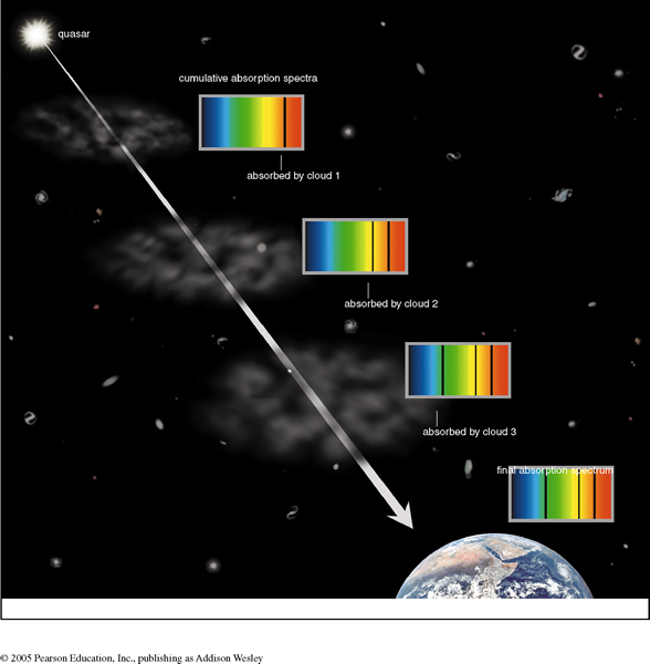
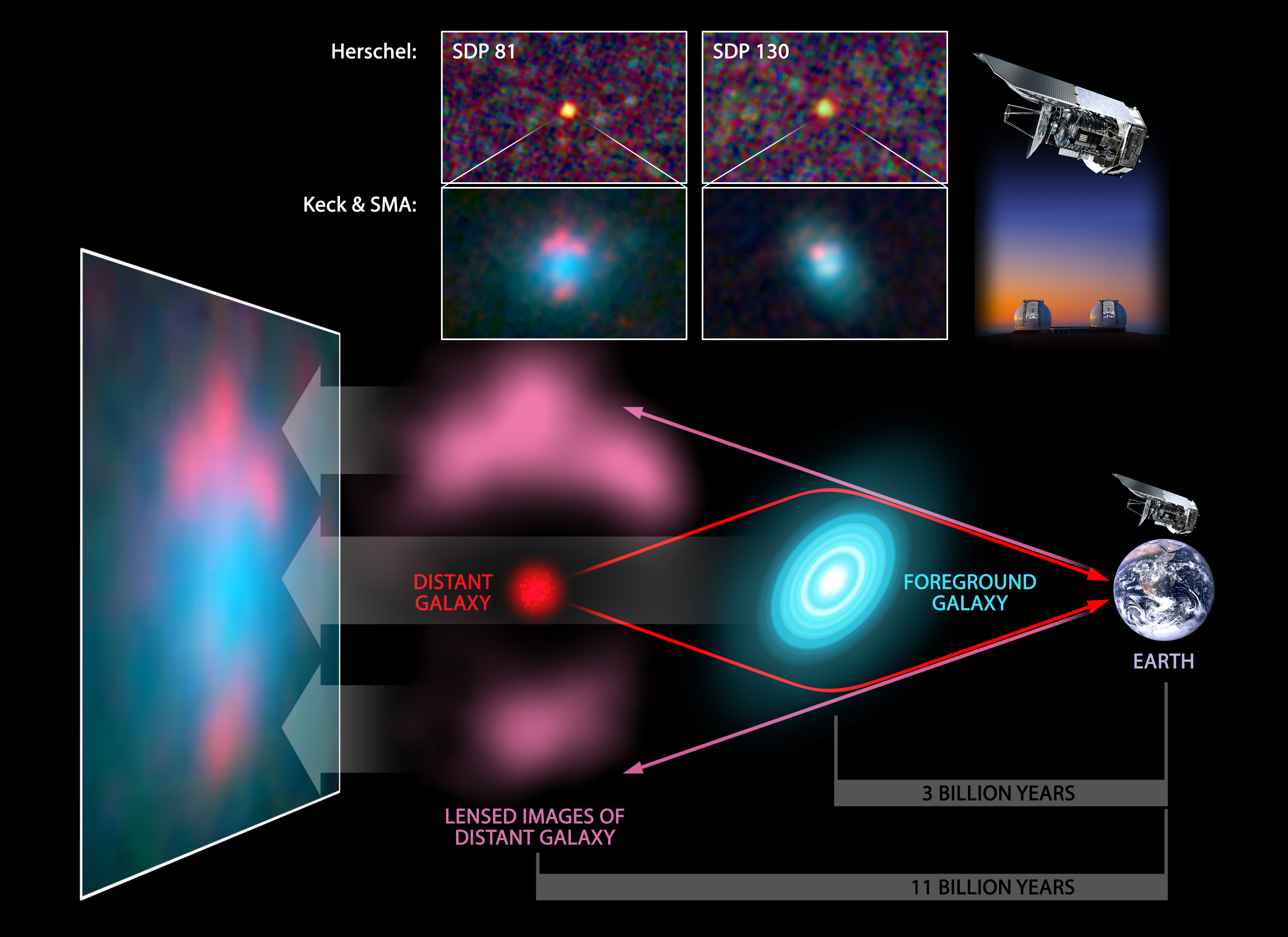
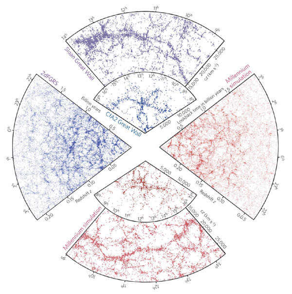
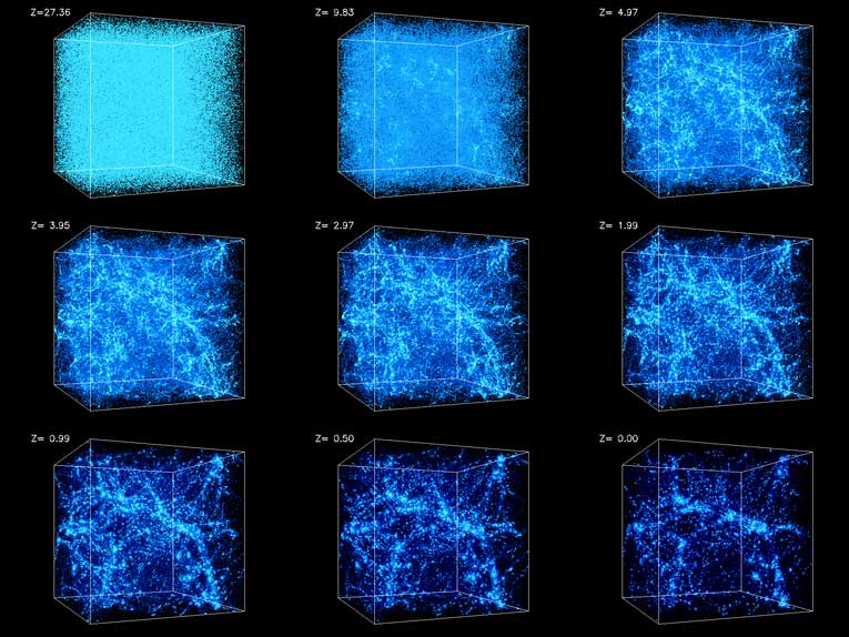
Stellar Mass and Surface Gravity
- The text transitions from measuring stellar distance and luminosity to the fundamental physical parameter of stellar mass.
- Newton's law of gravitation provides the mathematical framework for calculating surface gravity based on a star's mass and radius.
- The Sun's surface gravity is approximately 27 times that of Earth, significantly increasing the theoretical weight of any object on its surface.
- Red Giant stars possess extremely low surface gravity due to their massive expansion, often leading to the loss of their outer envelopes into space.
- Compact remnants like white dwarfs and neutron stars exhibit surface gravities thousands to millions of times stronger than the Sun due to their extreme density.
- Surface gravity serves as a precursor to understanding more complex concepts like escape velocity and orbital speeds in binary systems.
Imagine what you'd weigh then on the surface of a neutron star!
7 Surface Gravity and Escape/Orbital
Speed
So far we've been able to
nds ways to estimate the
rst
ve stellar parameters on
our list { distance, luminosity, temperature, radius, and elemental composition.
Moreover, we've done this with just a few, relatively simple measurements {
parallax, apparent magnitude, color, and spectral line patterns. But along the
way we've had to learn to exploit some key geometric principles and physical
laws { angular-size/parallax, inverse-square law, and Planck's, Wien's and the
Stefan-Boltzman laws of blackbody radiation.
So what of the next item on the list, namely stellar mass? Mass is clearly a
physically important parameter for a star, since for example it will help determine
the strength of the gravity that tries to pull the star's matter together. To lay
the groundwork for discussing one basic way we can determine mass (from orbits
of stars in stellar binaries), let's
rst review the Newton's law of gravitation and
show how this sets such key quantities like the surface gravity, and the speeds
required for material to escape or orbit the star.
7.1 Newton's law of gravitation and stellar surface gravity
On Earth, an object of mass mhas a weight given by
Fgrav=mge; (7.1)
where the acceleration of gravity on Earth is ge= 980cm=s2= 9:8m=s2. But
this comes from Newtons's law of gravity, which states that for two point masses
mandMseparated by a distance r, the attractive gravitational force between
them is given by
Fgrav=GMm
r2; (7.2)
where Newton's constant of gravity is G= 6:710�8cm3=g=s2. Remarkably,
when applied to spherical bodies of mass Mand
nite radius R, the same formula
works for all distances rRat or outside the surface!1Thus, we see that the
1Even more remarkably, even if we are inside the radius, r<R , then we can still use
Newton's law if we just count that part of the total mass that is insider, i.e.Mr, and
completely ignore all the mass that is above r.
38 Surface Gravity and Escape/Orbital Speed
acceleration of gravity at the surface of the Earth is just given by the mass and
radius of the Earth through
ge=GMe
R2e: (7.3)
Similarly for stars, the surface gravity is given by the stellar mass Mand radius
R. In the case of the Sun, this gives g
= 2:6104cm/s227ge. Thus, if you
could stand on the surface of the Sun, your \weight" would be about 27 times
what it is on Earth.
For other stars, gravities can vary over a quite wide range, largely because of
the wide range in size. For example, when the Sun get's near the end of its life
about 5 billion years from now, it will swell up to more than 100 times its current
radius, becoming what's known as a \Red Giant" ( x19). Stars we see now that
happen to be in this Red Giant phase thus tend to have quite low gravity, about
a fraction 1/10,000 that of the Sun.
Largely because of this very low gravity, much of the outer envelope of such
Red Giant stars will actually be lost to space (forming, as we shall see, quite
beautiful nebulae; see x19 and
gure 20.5.) When this happens to the Sun, what's
left behind will be just the hot stellar core, a so-called \white dwarf", with about
2/3 the mass of the current Sun, but with a radius only about that of the Earth,
i.e.RRe7103km0:01R
. The surface gravities of white dwarfs are
thus typically 10 ;000 times higher than the current Sun ( x19.4).
For \neutron stars", which are the remnants of stars a bit more massive than
the Sun, the radius is just about 10 km, more than another factor 500 smaller
than white dwarfs ( x20.3). This implies surface gravities another 5-6 orders of
magnitude higher than even white dwarfs. (Imagine what you'd weigh then on
the surface of a neutron star!)
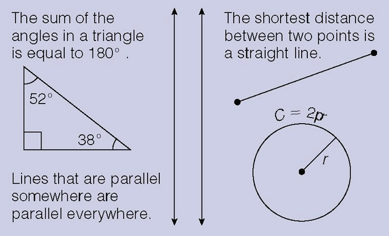
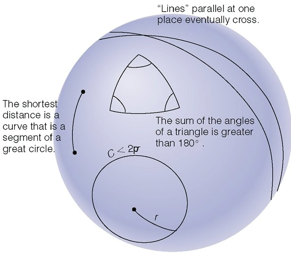
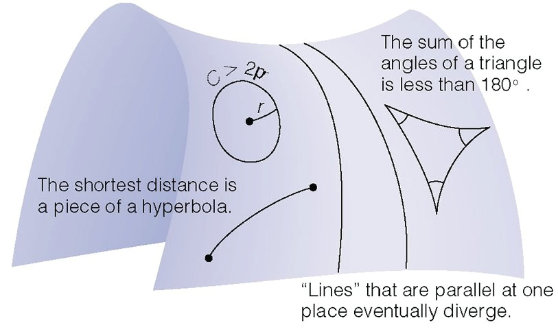
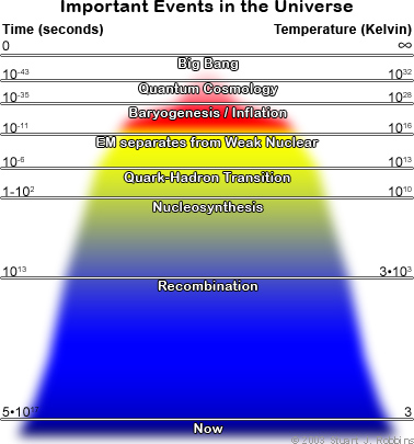
Gravity and Orbital Mechanics
- Stellar remnants like white dwarfs and neutron stars exhibit extreme surface gravities, with neutron stars reaching ten billion times the gravity of Earth.
- The log g scale provides a standardized way to compare gravitational strength across diverse celestial bodies, from Red Giants to dense stellar cores.
- Escape speed represents the velocity required for an object to overcome a body's gravitational pull and reach an infinite distance.
- Circular orbital speed is mathematically related to escape speed, specifically being the escape speed divided by the square root of two.
- The Virial Theorem establishes a fundamental relationship in bound orbits where kinetic energy is equal to half of the absolute gravitational binding energy.
Imagine what you'd weigh then on the surface of a neutron star!
left behind will be just the hot stellar core, a so-called \white dwarf", with about
2/3 the mass of the current Sun, but with a radius only about that of the Earth,
i.e.RRe7103km0:01R
. The surface gravities of white dwarfs are
thus typically 10 ;000 times higher than the current Sun ( x19.4).
For \neutron stars", which are the remnants of stars a bit more massive than
the Sun, the radius is just about 10 km, more than another factor 500 smaller
than white dwarfs ( x20.3). This implies surface gravities another 5-6 orders of
magnitude higher than even white dwarfs. (Imagine what you'd weigh then on
the surface of a neutron star!)
Since stellar gravities vary over such a large range, it is customary to quote
them in terms of the log of the gravity, log g, using CGS units. We thus have
gravities ranging from log g0 for Red Giants, to log g4 for normal stars
like the Sun, to log g8 for white dwarfs, to log g13 for neutron stars. Since
the Earth's gravity has log ge3, the di
erence of log gfrom 3 is the number of
order of magnitudes more/less that you'd weigh on that surface. For example,
for neutron stars the di
erence from Earth is 10, implying you'd weigh 1010, or
ten billion times more on a neutron star! On the other hand, on a Red Giant,
your weight would be about 1000 times lessthan on Earth.
7.2 Surface escape speed Vesc
Another measure of the strength of a gravitational
eld is through the surface
escape speed,
Vesc=r
2GM
R: (7.4)
7.3 Speed for circular orbit 39
A object of mass mlaunched with this speed has a kinetic energy mV2
esc=2 =
GMm=R . This just equals the work needed to lift that object from the surface
radiusRto escape at a large radius r!1 ,
W=Z1
RGMm
r2dr=GMm
R: (7.5)
Thus if one could throw a ball (or launch a rocket!) with this speed outward
from a body's surface radius R, then2by conservation of total energy, that ob-
ject would reach an arbitrarily large distance from the star, with however a
vanishingly small
nal speed.
For the earth, the escape speed is about 25,000 mph, or 11.2 km/s. By compar-
ison, for the moon, it is just 2.4 km/s, which is one reason the Apollo astronauts
could use a much smaller rocket to get back from the moon, than they used to
get there in the
rst place. However, escaping from the surface of the Sun (and
most any star), is much harder, requiring an escape speed of 618 km/s.
7.3 Speed for circular orbit
Let us next compare this escape speed with the speed needed for an object to
maintain a circular orbit at some radius rfrom the center a gravitating body of
massM. For an orbiting body of mass m, we require that the gravitational force
be balanced by the centrifugal force from moving along the circle of radius r,
GMm
r2=mV2
orb
r; (7.6)
which solves to
Vorb(r) =r
GM
r: (7.7)
Note in particular that the orbital speed very near the stellar surface, rR,
is given by Vorb(R) =Vesc=p
2. Thus the speed of satellites in low-earth-orbit
(LEO) is about 17,700 mph, or 7.9 km/s.
Of course, orbits can also be maintained at any radius above the surface radius,
r > R , and eqn. (7.7) shows that in this case, the speed needed declines as
1=pr. Thus, for example, the orbital speed of the earth around the Sun is about
30 km/s, a factor ofp
R
=au=p
1=215 = 0:0046 smaller than the orbital speed
near the Sun's surface, Vorb;
= 434 km/s.
7.4 Virial Theorum for bound orbits
If we de
ne the gravitational energy to be zero far from a star, then for an object
of massmat a radius rfrom a star of mass M, we can write the gravitational
2neglecting forces other than gravity, like the drag from an atmosphere
40 Surface Gravity and Escape/Orbital Speed
binding energy Uas the negative of the escape energy,
U(r) =�GMm
r: (7.8)
If this same object is in orbit at this radius r, then the kinetic energy of the orbit
is
T(r) =mV2
orb
2= +GMm
2r=�U(r)
2; (7.9)
where the second equation uses eqn. (7.7) for the orbital speed Vorb(r). We can
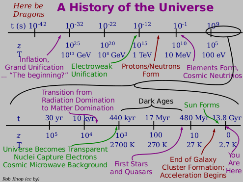
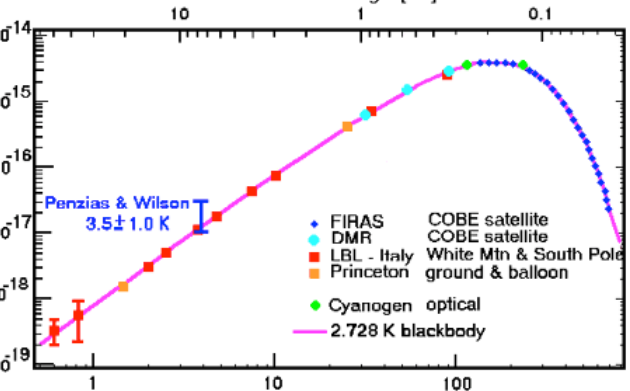
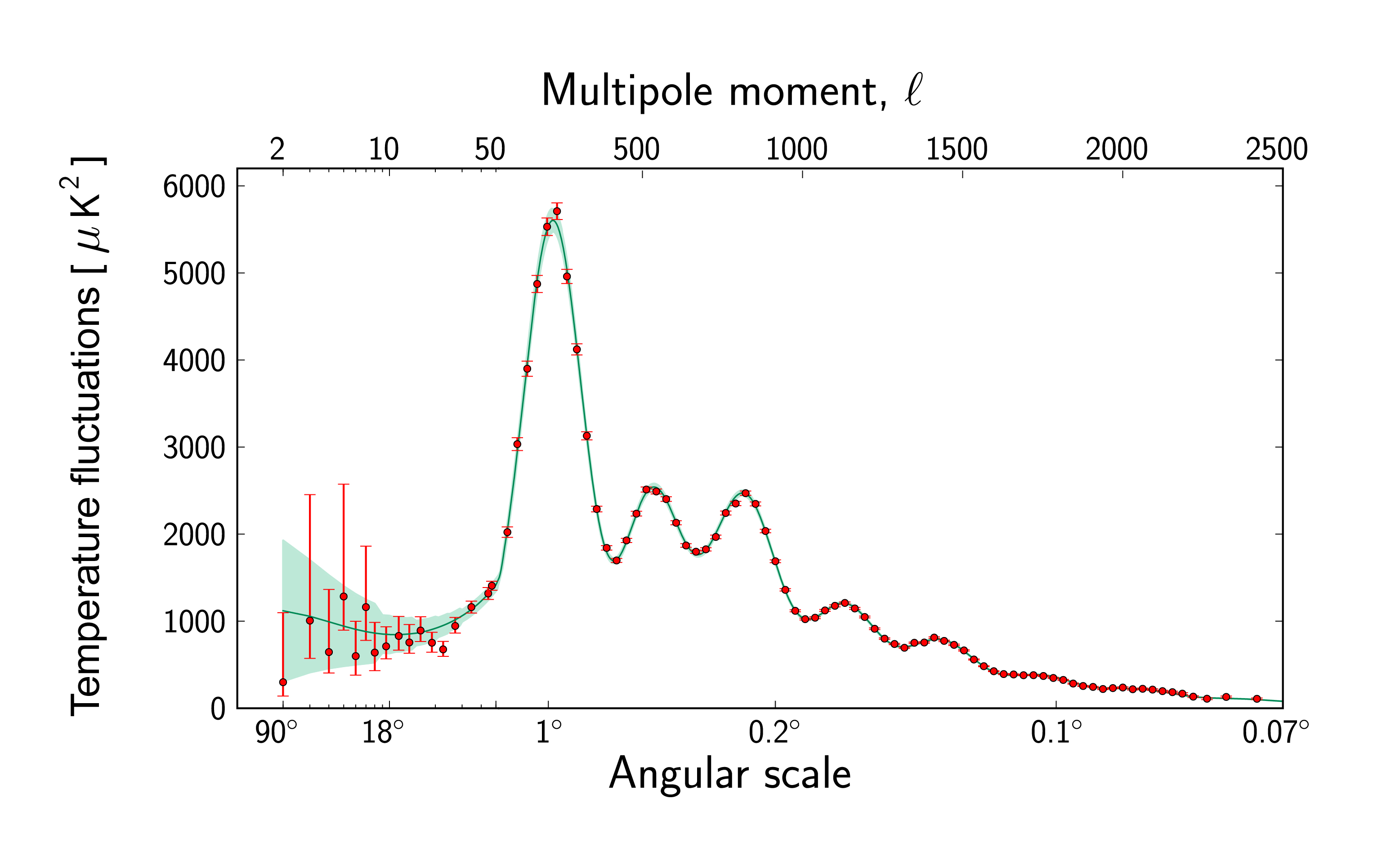
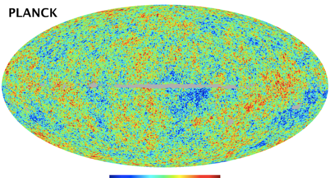
Gravitational Energy and the Virial Theorem
- The text defines gravitational binding energy as the negative of the energy required for an object to escape a star's pull.
- For a stable orbit, kinetic energy is shown to be exactly half of the absolute value of the gravitational binding energy.
- The Virial Theorem states that total energy in a stably bound system equals half of the gravitational binding energy, a principle applicable to both orbits and internal stellar structures.
- The theorem extends to stars by treating internal thermal energy as a form of kinetic energy that balances self-gravity.
- Mathematical exercises are provided to calculate surface gravity, escape speeds, and orbital velocities for various stellar masses and radii.
- The text transitions into the historical search for stellar energy sources, questioning if chemical burning could sustain a star's lifespan.
This fact that the total energy E just equals half the gravitational binding energy U is an example of what is known as the Virial Theorem.
ne the gravitational energy to be zero far from a star, then for an object
of massmat a radius rfrom a star of mass M, we can write the gravitational
2neglecting forces other than gravity, like the drag from an atmosphere
40 Surface Gravity and Escape/Orbital Speed
binding energy Uas the negative of the escape energy,
U(r) =�GMm
r: (7.8)
If this same object is in orbit at this radius r, then the kinetic energy of the orbit
is
T(r) =mV2
orb
2= +GMm
2r=�U(r)
2; (7.9)
where the second equation uses eqn. (7.7) for the orbital speed Vorb(r). We can
then write the total energy as
E(r)T(r) +U(r) =�T(r) =U(r)
2: (7.10)
This fact that the total energy Ejust equals halfthe gravitational binding energy
Uis an example of what is known as the Virial Theorum . It is applicable broadly
to most any stably bound gravitational system. For example, if we recognize that
the thermal energy inside a star as a kind of kinetic energy, it even applies to
stars, in which the internal gas pressure balances the star's own self gravity. This
is discussed further in x8.2 and the part II notes on stellar structure.
7.5 Questions and Exercises
Quick Question 1: In CGS units, the Sun has log g
4:44. Compute the log gfor
stars with:
a.M= 10M
andR= 10R
b.M= 1M
andR= 100R
c.M= 1M
andR= 0:01R
Quick Question 2:
The Sun has an escape speed of Ve
= 618 km/s. Compute the escape speed Veof
the stars in parts a-c of QQ1.
Quick Question 3:
The earth has an orbital speed of Ve= 2au/yr = 30 km/s. Compute the orbital
speedVorb(in km/s) of a body at the following distances from the stars with the quoted
masses:
a.M= 10M
andd= 10 au.
b.M= 1M
andd= 100 au.
c.M= 1M
andd= 0:01 au.
Exercise 1:
a. During a solar eclipse, the moon just barely covers the visible disk of the Sun.
What does this tell you about the relative angular size of the Sun and moon?
b. Given that the moon is at a distance of 0.0024 au, what then is the ratio of the
physical size of the moon vs. Sun?
7.5 Questions and Exercises 41
c. Compared to earth, the Sun and moon have gravities of respectively 27 geand
ge=6. Using this and your answer above, what is the ratio of the mass of the moon to
that of the Sun?
d. Using the above, plus known values for Newton's constant G, earth's gravity
ge= 9:8 m/s2, and the solar radius R
= 700;000 km, compute the masses of the Sun
and moon in kg.
Exercise 2:
a. What is the ratio of the energy needed to escape the moon vs. the earth? What's
the ratio for the Sun vs. the earth?
b. What is the escape speed (in km/s) from a star with: (1) M= 10M
andR=
10R
; (2)M= 1M
andR= 100R
; (3)M= 1M
andR= 0:01R
?
c. To what radius (in km) would you have to shrink the Sun to make its escape speed
equal to the speed of light c?
Exercise 3:
a. What is the ratio of the energy needed to escape the the earth vs. that needed to
reach LEO?
b. What is the orbital speed (in km/s) of a planet that orbits at a distance afrom a
star with mass M, given: (1) M= 10M
anda= 10 au; (2) M= 1M
anda= 100;
au; (3)M= 1M
anda= 0:01 au?
8 Stellar Ages and Lifetimes
In our list of basic stellar properties, let us next consider stellar age. Just how
old are stars like the Sun? What provides the energy that keeps them shining?
And what will happen to them as they exhaust various available energy sources?
8.1 Shortness of chemical burning timescale for Sun and stars
When 19th century scientists pondered the possible energy sources for the Sun,
some
rst considered whether this could come from the kind of chemical reactions
(e.g., from fossil fuels like coal, oil, natural gas, etc.) that power human activities
on Earth. But such chemical reactions involve transitions of electrons among
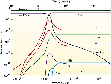
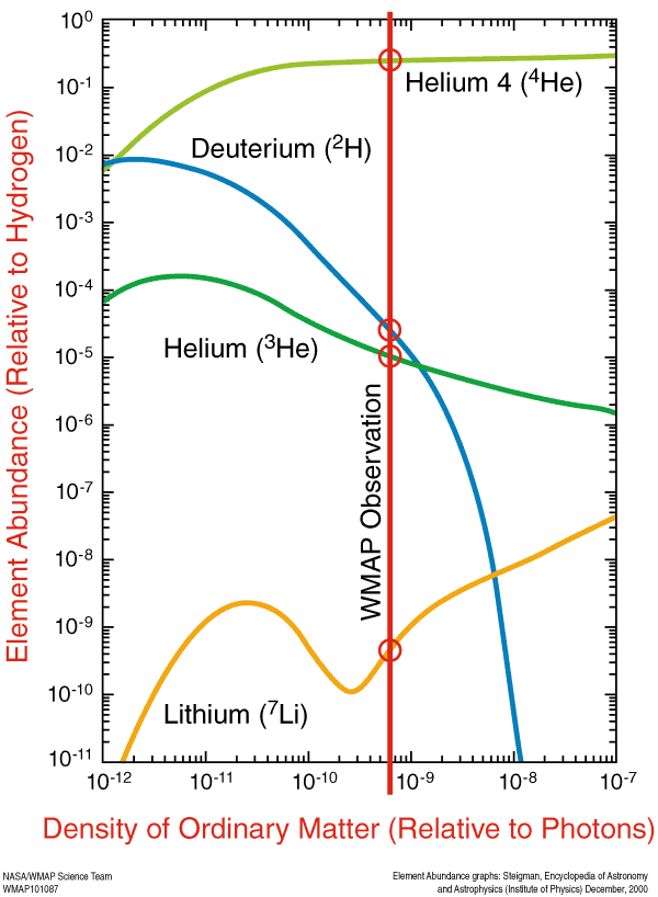
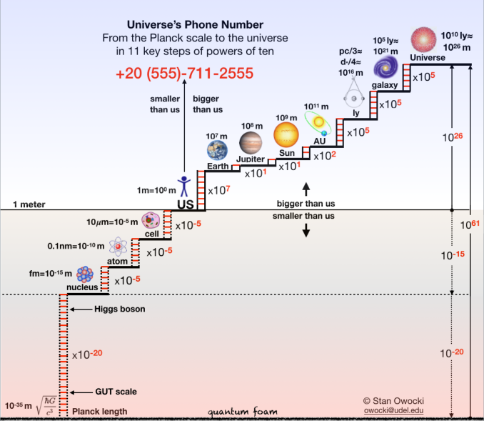
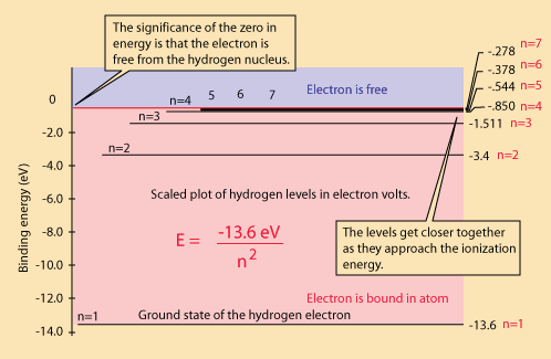
Stellar Energy and Timescales
- Nineteenth-century scientists initially explored chemical reactions as a solar energy source but found they could only power the Sun for about 15,000 years.
- The Kelvin-Helmholtz timescale suggests that gravitational contraction could power the Sun for 30 million years by converting potential energy into radiation.
- Geological evidence of the Earth's age eventually proved that both chemical and gravitational energy sources are insufficient to explain solar longevity.
- Nuclear fusion provides the actual energy source, operating with a mass-energy efficiency roughly seven million times greater than chemical reactions.
- By fusing hydrogen into helium in its core, a star like the Sun can maintain its luminosity for approximately 10 billion years.
Even in the 19th century, it was clear, e.g. from geological processes like erosion, that the Earth — and so presumably also the Sun — had to be much older than this.
In our list of basic stellar properties, let us next consider stellar age. Just how
old are stars like the Sun? What provides the energy that keeps them shining?
And what will happen to them as they exhaust various available energy sources?
8.1 Shortness of chemical burning timescale for Sun and stars
When 19th century scientists pondered the possible energy sources for the Sun,
some
rst considered whether this could come from the kind of chemical reactions
(e.g., from fossil fuels like coal, oil, natural gas, etc.) that power human activities
on Earth. But such chemical reactions involve transitions of electrons among
various bound states of atoms, and, as discussed below ( xA.1) for the Bohr
model of the Hydrogen, the scale of energy release in such transitions is limited
to something on the order of an electron volt (eV). In contrast, the rest-mass
energy of the protons and neutrons that make up the mass is about 1 GeV, or
109times higher. With the associated mass-energy eciency of 10�9, we can
readily estimate a timescale for maintaining the solar luminosity from chemical
reactions,
tchem =M
c2
L
=4:51020s =1:51013yr15;000 yr: (8.1)
Even in the 19th century, it was clear, e.g. from geological processes like erosion,
that the Earth { and so presumably also the Sun { had to be much older than
this.
8.2 Kelvin-Helmholtz timescale for gravitational contraction
So let us consider whether, instead of chemical reactions, gravitational contrac-
tion might provide the energy source to power the Sun and other stars. As a star
undergoes a contraction in radius, its gravitational binding becomes stronger,
with a deeper gravitational potential energy, yielding an energy release set by
the negative of the change in gravitational potential ( �dU > 0). If the contrac-
tion is gradual enough that the star roughly maintains dynamical equilibrium,
8.3 Nuclear burning timescale 43
then just half of the gravitational energy released goes into heating up the star1,
leaving the other half available to power the radiative luminosity, L=�1
2dU=dt .
For a star of observed luminosity Land present-day gravitational binding energy
U, we can thus de
ne a characteristic gravitational contraction lifetime,
tgrav=�1
2U
LtKH (8.2)
where the subscript \KH" refers to Kelvin and Helmholtz, the names of the
two scientists credited with
rst identifying this as an important timescale. To
estimate a value for the gravitational binding energy, let us consider the example
for the Sun under the somewhat arti
cial assumption that it has a uniform,
constant density, given by its mass over volume, =M
=(4R3
=3). Since the
gravity at any radius rdepends only on the mass m=4r3=3inside that
radius, the total gravitational binding energy of the Sun is given by integrating
the associated local gravitational potential �Gm=r over all di
erential mass
shellsdm,
�U=ZM
0Gm
rdm=162
3G2ZR
0r4dr=3
5GM2
R
; (8.3)
Applying this in eqn. (8.2), we
nd for the \Kelvin-Helmholtz" time of the
Sun,
tKH3
10GM2
R
L
30 Myr: (8.4)
Although substantially longer than the chemical burning timescale (8.1), this
is still much shorter than the geologically inferred minimum age of the Earth,
which is several Billion years.
8.3 Nuclear burning timescale
We now realize, of course, that the ages and lifetimes of stars like the Sun are set
by a much longer nuclear burning timescale. When four hydrogen nuclei are fused
into a helium nucleus, the helium mass is about 0 :7%lower than the original four
hydrogen. For nuclear fusion the above-de
ned mass-energy burning eciency
is thus now nuc0:007. But in a typical main sequence star, only some core
fractionf1=10 of the stellar mass is hot enough to allow Hydrogen fusion.
Applying this we thus
nd for the nuclear burning timescale
tnuc=nucfMc2
L10 GyrM=M
L=L
; (8.5)
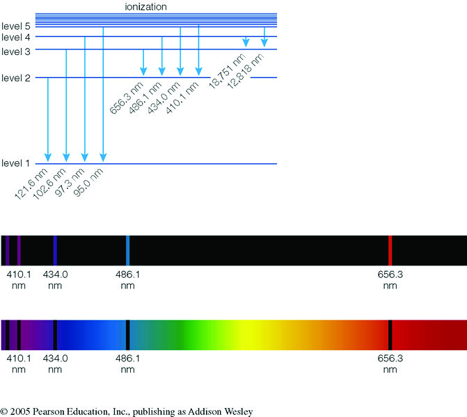
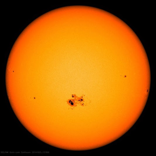
Stellar Lifetimes and Cluster Ages
- The Sun's lifetime is determined by nuclear fusion efficiency, where 0.7% of mass is converted to energy, giving it a total lifespan of approximately 10 billion years.
- Currently 4.6 billion years old, the Sun is roughly halfway through its hydrogen-burning phase before it will exhaust its core fuel.
- Stellar luminosity scales steeply with mass (L ~ M³), meaning high-mass stars consume their fuel much faster and have significantly shorter lifespans than low-mass stars.
- The most massive stars may live for only 1 million years, a stark contrast to the multi-billion-year timescales of solar-mass stars.
- The age of a stellar cluster can be determined by identifying the 'turn-off point' on an H-R diagram, where stars begin to exhaust their hydrogen and exit the main sequence.
The most massive stars, of order 100 M, and thus with luminosities of order 106L, have main-sequence lifetimes of only about about 1 Myr, much shorter the multi-Gyr timescale for solar-mass stars.
We now realize, of course, that the ages and lifetimes of stars like the Sun are set
by a much longer nuclear burning timescale. When four hydrogen nuclei are fused
into a helium nucleus, the helium mass is about 0 :7%lower than the original four
hydrogen. For nuclear fusion the above-de
ned mass-energy burning eciency
is thus now nuc0:007. But in a typical main sequence star, only some core
fractionf1=10 of the stellar mass is hot enough to allow Hydrogen fusion.
Applying this we thus
nd for the nuclear burning timescale
tnuc=nucfMc2
L10 GyrM=M
L=L
; (8.5)
where Gyr109yr, i.e., a billion years, or a \Giga-year".
1This is another example of the Virial theorem for gravitationally bound systems, as
discussed in 7.4.
44 Stellar Ages and Lifetimes
We thus see that the Sun can live for about 10 Gyr by burning Hydrogen into
Helium in its core. It's present age of 4.6 Gyr2thus puts it roughly half way
through this Hydrogen-burning phase, with about 5.4 Gyr to go before it runs
out of H in its core.
8.4 Age of stellar clusters from main-sequence turno
point
As discussed below (see x10.4 and eqn. 10.11), observations of stellar binary
systems indicate that the luminosities of main-sequence stars scale with a high
power of the stellar mass { roughly LM3. In the present context, this implies
that high-mass stars should have much shorter lifetimes than low-mass stars.
If we make the reasonable assumption that the same
xed fraction ( f0:1) of
the total hydrogen mass of any star is available for nuclear burning into helium in
its stellar core, then the fuel available scales with the mass, while the burning rate
depends on the luminosity. Normalized to the Sun, the main-sequence lifetime
thus scales as
tms=tms;
M=M
L=L
10 GyrM
M2
: (8.6)
The most massive stars, of order 100 M
, and thus with luminosities of order
106L
, have main-sequence lifetimes of only about about 1 Myr, much shorter
the multi-Gyr timescale for solar-mass stars.
Figure 8.1 Left: H-R diagram for globular cluster M55, showing how stars on the
upper main sequence have evolved to lower temperature giant stars. Right: Schematic
H-R diagram for clusters, showing the systematic peeling o
of the main sequence
with increasing cluster age.
2As inferred, e.g., from radioactive dating of the oldest meteorites.
8.5 Questions and Exercises 45
This strong scaling of lifetime with mass can be vividly illustratied by plotting
the H-R diagram of stellar clusters. The H-R diagram plotted in
gure 6.5 is for
volume-limited sample near the Sun, consisting of stars of a wide range of ages,
distances, and perhaps even chemical composition. But stars often appear in
clusters, all roughly at the same distance, and, since they likely formed over a
relatively short time span out of the same interstellar cloud, they all have roughly
the same age and chemical composition. Using eqn. (8.6) together with the the
LM3relation, the age of a stellar cluster can be inferred from its H-R diagram
simply by measuring the luminosity Ltoof stars at the \ turn-o
" point from the
main sequence,
tcluster10 GyrL
Lto2=3
: (8.7)
The left panel of
gure 8.1 plots an actual H-R diagram for the globular cluster
M55. Note that stars to the upper left of the main sequence have evolved to a
vertical branch of cooler stars extending up to the Red Giants3. This re
ects the
fact that more luminous stars exhaust their hydrogen fuel sooner that dimmer
stars, as shown by the inverse luminosity scaling of the nuclear burning timescale
in eqn. (8.5). The right panel illustrates schematically the H-R diagrams for
various types of stellar clusters, showing how the turno
point from the main
sequence is an indicator of the cluster age. Observed cluster H-R diagrams like
this thus provide a direct diagnostic of the formation and evolution of stars with
various masses and luminosities.
8.5 Questions and Exercises
Stellar Lifetimes and Space Velocities
- The main-sequence turn-off point in H-R diagrams serves as a critical diagnostic for determining the age of stellar clusters.
- Luminous stars exhaust their hydrogen fuel significantly faster than dimmer stars due to inverse luminosity scaling.
- Blue stragglers are stars rejuvenated by mass transfer from a binary companion, making them appear younger and hotter than their peers.
- Stellar motion is measured through proper motion (transverse drift) and spectrometric techniques for radial velocity.
- Barnard's star exhibits the highest proper motion of any star, showing a detectable drift even with modest equipment.
This rejuvenated the mass gainer, making it again a hot, luminous blue star.
fact that more luminous stars exhaust their hydrogen fuel sooner that dimmer
stars, as shown by the inverse luminosity scaling of the nuclear burning timescale
in eqn. (8.5). The right panel illustrates schematically the H-R diagrams for
various types of stellar clusters, showing how the turno
point from the main
sequence is an indicator of the cluster age. Observed cluster H-R diagrams like
this thus provide a direct diagnostic of the formation and evolution of stars with
various masses and luminosities.
8.5 Questions and Exercises
Quick Question 1: What are the luminosities (in L
) and the expected main sequence
lifetimes (in Myr) of stars with masses: a. 10 M
? b. 0.1M
? c. 100M
?
Quick Question 2: Suppose you observe a cluster with a main-sequence turno
point
at a luminosity of 100 L
. What is the cluster's age, in Myr. What about for a cluster
with a turno
at a luminosity of 10 ;000L
?
Exercise 1: A cluster has a main-sequence turno
at a spectral type G2, corresponding
to stars of apparent magnitude m= +10.
(a) About what is the luminosity, in L
, of the stars at the turno
point?
(b) About what is the age (in Gyr) of the cluster?
(c) About what is the distance (in pc) of the cluster?
3Stars just above this main sequence turn-o
are dubbed \blue stragglers". They are stars
whose close binary companion became a Red Giant with a such big radius that mass from
its envelope spilled over onto it. This rejuvenated the mass gainer, making it again a hot,
luminous blue star.
46 Stellar Ages and Lifetimes
Exercise 2: Con
rm the integration result in eqn. (8.3).
9 Inferring Stellar Space Velocities
The next section ( x10) will use the inferred orbits of stars in binary star systems
to directly determine stellar masses. But
rst, as a basis for interpreting obser-
vations of such systems in terms of the orbital velocity of the component stars,
let us review the astrometric and spectrometric techniques used to measure the
motion of stars through space.
9.1 Transverse speed from proper motion observations
In addition to such periodic motion from binary orbits, stars generally also ex-
hibit some systematic motion relative to the Sun, generally with components
both transverse (i.e. perpendicular) to and along (parallel to) the observed line
of sight. For nearby stars, the perpendicular movement, called \proper motion",
can be observed as a drift in the apparent position in the star relative to the
more
xed pattern of more distant, background stars. Even though the associ-
ated physical velocities can be quite large, e.g. Vt10�100 km/s, the distances
to stars is so large that proper motions of stars { measured as an angular drift
per unit time, and generally denoted with the symbol { are generally no bigger
than about 1 arcsec/year. But because this is a systematic drift, the longer
the star is monitored, the smaller the proper motion that can be detected, down
to about1 arcsec/century or less for the most well-observed stars.
Figure 9.1 illustrates the proper motion for Barnard's star, which has the
highestvalue of any star in the sky. It is so high in fact, that its proper motion
can even be followed with a backyard telescope, as was done for this
gure. This
star is actually tracking along the nearly South-to-North path labeled as the
\Hipparcos1mean" in the
gure. The apparent, nearly East-West (EW) wobble
is due to the Earth's own motion around the Sun, and indeed provides a measure
of the star's parallax, and thus its distance. Referring to the arcsec marker in
the lower right, we can estimate the full amplitude of the wobble at a bit more
than an arcsec, meaning the parallax2isp0:55 arcsec, implying a distance
1Hipparcos is an orbiting satellite that, because of the absence of the atmospheric blurring,
can make very precise \astrometric" measurements of stellar positions, at precisions
Measuring Stellar Space Velocities
- The apparent wobble in a star's path, such as Barnard's star, is caused by Earth's orbital motion and provides a direct measure of stellar parallax.
- Stellar distance can be calculated from parallax, which then allows astronomers to convert observed proper motion into a physical transverse velocity.
- Barnard's star exhibits one of the fastest transverse speeds among nearby stars, moving at approximately 90 km/s.
- Radial velocity, the component of motion along the line of sight, is measured using the Doppler effect rather than direct positional shifts.
- The Doppler effect causes a shift in observed wavelength proportional to the object's speed relative to the speed of the signal, such as light or sound.
- In extreme cases where an object moves faster than the signal speed, such as supersonic travel, shock waves like sonic booms are created.
Consider the noise from a car on a highway, for which the 'vvvvrrrrrooomm' sound stems from just this shift in pitch from the car engine noise.
gure. The apparent, nearly East-West (EW) wobble
is due to the Earth's own motion around the Sun, and indeed provides a measure
of the star's parallax, and thus its distance. Referring to the arcsec marker in
the lower right, we can estimate the full amplitude of the wobble at a bit more
than an arcsec, meaning the parallax2isp0:55 arcsec, implying a distance
1Hipparcos is an orbiting satellite that, because of the absence of the atmospheric blurring,
can make very precise \astrometric" measurements of stellar positions, at precisions
approaching a milli-arcsec.
2given by half the full amplitude, since parallax assumes a 1 au baseline that is half the full
diameter of earth's orbit
48 Inferring Stellar Space Velocities
Figure 9.1 Proper motion of Barnard's star. The star is actually tracking along the
path labeled as the mean from the Hipparcos astrometric satellite. The apparent
wobble is due to the parallax from the Earth's own motion around the Sun. Referring
to lower right label showing one arcsec, we can estimate the full amplitude of the
parallax wobble as about 1.1 arcsec; but since this re
ects a baseline of 2 AU from
the earth's orbital diameter, the (one-AU) parallax angle is half this, or
p= 0:55 arcsec, implying a distance of d= 1=p1:8 pc.
ofd1:8 pc. By comparison, the roughly South-to-North proper motion has a
value10 arcsec/yr.
In general, with a known parallax pin arcsec, and known proper motion in
arcsec/yr, we can derive the associated transverse velocity Vtacross our line of
sight,
Vt=
pau=yr = 4:7
pkm=s; (9.1)
where the last equality uses the fact that the Earth's orbital speed VE= 2au=yr =
30 km/s. For Barnard's star this works out to give Vt90 km/s, or about 3
times the earth's orbital speed around the Sun. This among the fastest trans-
verse speeds inferred among the nearby stars.
9.2 Radial velocity from Doppler shift 49
9.2 Radial velocity from Doppler shift
We've seen how we can directly measure the transverse motion of relatively
nearby, fast-moving stars in terms of their proper motion. But how might we
measure the radial velocity component along our line of sight? The answer is:
via the \Doppler e
ect", wherein such radial motion leads to an observed shift
in the wavelength of the light.
To see how this e
ect comes about, we need only consider some regular signal
with period Pobeing emitted from an object moving at a speed Vrtoward
(Vr<0) or away ( Vr>0) from us. Let the signal travel at a speed Vs, where
Vs=cfor a light wave, but might equally as well be speed of sound if we were
to use that as an example. For clarity of language, let us assume the object is
moving away, with Vr>0. Then after any given pulse of the signal is emitted,
the object moves a distance VrPobefore emitting the next pulse. Since the pulse
still travels at the same speed, this implies it takes the second pulse an extra
time
P=VrPo
Vs(9.2)
to reach us. Thus the period we observe is longer, P0=Po+ P.
For a wave, the wavelength is given by =PVs, implying then an associated
stretch in the observed wavelength
0=P0Vs= (Po+ P)Vs= (Vs+Vr)Po=o+VrPo: (9.3)
whereo=PoVsis the rest wavelength. The associated relative stretch in wave-
length is thus just
o0�o
o=Vr
Vs: (9.4)
For sound waves, this formula works in principle as long as Vr>�Vs. But if
an object moves toward us faster than sound ( Vr<�Vs), then it can basically
\overrun" the signal. This leads to strongly compressed sound waves, called
\shock waves", which are the basic origin of the sonic boom from a supersonic
jet. For some nice animations of this, see
http://www.lon-capa.org/ mmp/applist/doppler/d.htm
A common example of the Doppler e
ect in sound is the shift in pitch we hear
as the object moves past us. Consider the noise from a car on a highway, for
which the \vvvvrrrrrooomm" sound stems from just this shift in pitch from the
car engine noise. Figure 9.2 illustrates this for a racing car.
Doppler Shifts and Binary Systems
- The Doppler effect explains how sound waves compress into shock waves, creating sonic booms from supersonic jets.
- In astronomy, the Doppler shift of light allows scientists to measure a star's radial velocity by observing changes in spectral line wavelengths.
- Combining radial velocity with tangential velocity allows for the calculation of a star's total space velocity relative to the Sun.
- Barnard's star serves as a primary example of high space velocity, moving at 143 km/s toward our solar system.
- Binary star systems are so prevalent in the galaxy that astronomers jokingly claim 'three out of every two stars' are part of a binary.
- Binary systems are categorized as visual binaries, which are resolved through position monitoring, or spectroscopic binaries, which are identified via light spectra.
It turns out, in fact, that stellar binary (and even triple and quadruple) systems are quite common, so much so that astronomers sometimes joke that 'three out of every two stars is (in) a binary'.
\overrun" the signal. This leads to strongly compressed sound waves, called
\shock waves", which are the basic origin of the sonic boom from a supersonic
jet. For some nice animations of this, see
http://www.lon-capa.org/ mmp/applist/doppler/d.htm
A common example of the Doppler e
ect in sound is the shift in pitch we hear
as the object moves past us. Consider the noise from a car on a highway, for
which the \vvvvrrrrrooomm" sound stems from just this shift in pitch from the
car engine noise. Figure 9.2 illustrates this for a racing car.
In the case of light Vs=c, and so we can de
ne the Doppler shift of light as
o=Vr
c;jVrj
c: (9.5)
This assumes the non-relativistic case that jVrj
c, which applies well to most
all stellar motions. Straightforward observations of the associated wavelengths of
50 Inferring Stellar Space Velocities
Figure 9.2 Illustration of the Doppler shift of the sound from a racing car.
spectral lines in the star's spectrum relative to their rest (laboratory measured)
wavelengths thus gives a direct measurement of the star's motion toward or away
from the observer.
For our above example of Barnard's star, observations of the stellar spectrum
show a constant blueshift of ==�3:710�4, implying the star is moving
toward us, with a speed Vr=zc=�111 km/s. This allows us to derive the
overall space velocity ,
V=q
V2r+V2
t: (9.6)
For Barnard's star, this gives V= 143 km/s, which again is one of the highest
space velocities among nearby stars. Mapping the space motion of nearby stars
relative to the Sun provides some initial clues about the kinematics of stars in
our local region of the Milky Way galaxy.
9.3 Questions and Exercises
Quick Question 1: A star with parallax p= 0:02 arcsec is observed over 10 years to
have shifted by 2 arcsec from its proper motion. Compute the star's tangential space
velocityVt, in km/s.
Quick Question 2: For the star in QQ#1, a line with rest wavelength o= 600:00 nm
is observed to be at a wavelength = 600:09 nm.
a. Is the star moving toward us or away from us?
b. What is the star's Doppler shift z?
c. What is the star's radial velocity Vr, in km/s?
d. What is the star's total space velocityVtot, in km/s?
10 Using Binary Systems to Determine
Masses and Radii
Let us next consider how we can infer the masses of stars, namely through the
study of stellar binary systems .
It turns out, in fact, that stellar binary (and even triple and quadruple) systems
are quite common, so much so that astronomers sometimes joke that \three out
of every two stars is (in) a binary". The joke here works because often two
stars in a binary are so close together on the sky that we can't actually resolve
one star from another, and so we sometimes mistake the light source as coming
from a single star, when in fact it actually comes from two (or even more).
But even in such close binaries, we can often still tell there are two stars by
carefully studying the observed spectrum, and in this case, we call the system a
\spectroscopic binary" (see the next subsection, and
gure 10.2).
But for now, let's
rst focus on the simpler example of \visual binaries", a.k.a.
\astrometric" binaries (see
gure 10.1), since their detection typically requires
precise astrometric measurements of small variations of their positions on the
sky over time.
10.1 Visual binaries
In visual binaries, monitoring of the stellar positions over years and even decades
reveals that the two stars are actually moving around each other, much as the
Earth moves around the Sun. Figure 10.1 illustrates the principles behind visual
Measuring Mass in Visual Binaries
- Visual or astrometric binaries are detected by monitoring the precise movements of two stars as they orbit a common center of mass over years or decades.
- By combining the observed angular separation with the system's distance via parallax, astronomers can determine the physical distance between the stars.
- Unlike planetary systems where the central mass is dominant, binary stars often have comparable masses, requiring both to be treated as moving around a shared center of mass.
- Newton's generalization of Kepler's Third Law allows for the calculation of the total system mass based on the orbital period and the physical separation.
- If the individual orbital distances of both stars can be measured, the specific mass ratio and individual masses of each star can be calculated in solar units.
In visual binaries, monitoring of the stellar positions over years and even decades reveals that the two stars are actually moving around each other, much as the Earth moves around the Sun.
But for now, let's
rst focus on the simpler example of \visual binaries", a.k.a.
\astrometric" binaries (see
gure 10.1), since their detection typically requires
precise astrometric measurements of small variations of their positions on the
sky over time.
10.1 Visual binaries
In visual binaries, monitoring of the stellar positions over years and even decades
reveals that the two stars are actually moving around each other, much as the
Earth moves around the Sun. Figure 10.1 illustrates the principles behind visual
binaries. The time it takes the stars to go around a full cycle, called the orbital
period, can then be measured quite directly. Then if we can convert the apparent
angular separation into a physical distance apart { e.g. if we know the distance
to the system independently through a measured annual parallax for the stars in
the system { then we can use Kepler's 3rd law of orbital motion (as generalized
by Newton) to measure the total mass of the two stars.
It's actually quite easy to derive the full formula in the simple case of circular
orbits that lie in a plane perpendicular to our line of sight. For stars of mass M1
andM2separated by a physical distance a, Newton's law of gravity gives the
attractive force each star exerts on the other,
Fg=GM 1M2
a2: (10.1)
52 Using Binary Systems to Determine Masses and Radii
Figure 10.1 Illustration of the properties of a visual binary system.
A key di
erence from the case of a satellite orbiting the earth, or a planet orbiting
a star, is that in binary stars, the masses can become comparable. In this case,
each star (1,2) now moves around the center of mass at a
xed distance a1and
a2, with their ratio given by a2=a1=M1=M2and their sum by a1+a2=a. In
terms of the full separation, the orbital distance of, say, star 1 is thus given by
a1=aM2
M1+M2: (10.2)
For the given period P, the associated orbital speeds for star 1 is is given by
V1= 2a1=P. For a stable, circular orbit, the outward centrifugal force on star
1,
Fc1=M1V2
1
a1=42M1a1
P2=42a
P2M1M2
M1+M2; (10.3)
must balance the gravitational force from eqn. (10.1), yielding
GM 1M2
a2=42a
P2M1M2
M1+M2: (10.4)
This can be used to obtain the sum of the masses,
M1+M2=42
Ga3
P2=a3
au
P2yrM
; (10.5)
where the latter equality shows that evaluating the distance in au and the period
10.2 Spectroscopic binaries 53
in years gives the mass in units of the solar mass. For a visual binary in which we
can actually see both stars, we can separately measure the two orbital distances,
yielding then the mass ratio M2=M1=a1=a2. The mass for, e.g., star 1 is thus
given by
M1=a3
au
(1 +a1=a2)P2yrM
: (10.6)
The mass for star 2 can likewise be obtained if we just swap subscripts 1 and 2.
Equations (10.5) and (10.6) are actually forms of Kepler's 3rd law for planetary
motion around the Sun. Setting M1=M
and the planetary mass M2, we
rst
note that for all planets the mass is much smaller than for the Sun, M2=M1=
a1=a2
1, implying that the Sun only slightly wobbles (mostly to the counter
the pull of the most massive planet, namely Jupiter), with the planets thus pretty
much all orbiting around the Sun. If we thus ignore M2and plug in M1=M
in eqn. (10.5), we recover Kepler's third law in (almost) the form in which he
expressed it,
P2
yr=a3
au: (10.7)
To be precise, Kepler showed that in general the orbits of the planets are actually
ellipses , but this same law applies in that case we if we replace the circular orbital
distanceawith the \semi-major axis" of the ellipse. A circle is just a special case
of an ellipse, with the semi-major axis just equal to the radius.
In general, of course, real binary systems often have elliptical orbits, which,
Spectroscopic Binaries and Orbital Mechanics
- Kepler's third law applies to both circular and elliptical orbits by substituting the radius with the semi-major axis.
- Spectroscopic binaries are systems where stars are too close to resolve visually but can be identified via periodic Doppler shifts in their spectral lines.
- The inclination of an orbital plane can be disentangled from its ellipticity by observing the rate of movement along the projected orbit.
- In double-line spectroscopic binaries, the ratio of the stars' velocity amplitudes directly reveals their mass ratio.
- Newton's generalization of Kepler's third law allows for the calculation of individual stellar masses using orbital periods and radial velocities.
However, if the orbital plane is not perpendicular to the line of sight, then the orbital velocities of the stars will give a variable Doppler shift to each star's spectral lines.
in eqn. (10.5), we recover Kepler's third law in (almost) the form in which he
expressed it,
P2
yr=a3
au: (10.7)
To be precise, Kepler showed that in general the orbits of the planets are actually
ellipses , but this same law applies in that case we if we replace the circular orbital
distanceawith the \semi-major axis" of the ellipse. A circle is just a special case
of an ellipse, with the semi-major axis just equal to the radius.
In general, of course, real binary systems often have elliptical orbits, which,
moreover, lie in planes that are not always normal to the observer line of sight.
These systems can still be fully analyzed using the elliptical orbit form of New-
ton's generalization of Kepler's 3rd law, as derived, e.g. in Ch. 4 of the Astro 45
notes by Bill Press:
http://www.lanl.gov/DLDSTP/ay45/ay45c4.pdf
Indeed, by watching the rate of movement of the stars along the projected orbit,
the inclination e
ect can even be disentangled from the ellipticity.
10.2 Spectroscopic binaries
As noted, there are many stellar binary systems in which the angular separation
between the components is too close to readily resolve visually. However, if the
orbital plane is not perpendicular to the line of sight, then the orbital velocities
of the stars will give a variable Doppler shift to each star's spectral lines. The
e
ect is greatest when the orbits are relatively close , and in a plane containing
the line of sight, conditions which make such spectroscopic binaries complement
the wide visual binaries discussed above. Figure 10.2 illustrates the basic features
of a spectroscopic binary system.
If the two stars are not too di
erent in luminosity, then observations of the
combined stellar spectrum show spectral line signatures of both stellar spectra.
54 Using Binary Systems to Determine Masses and Radii
Figure 10.2 Illustration of the periodic Doppler shift of spectral lines in a
spectroscopic binary system.
As the stars move around each other in such \double-line" spectroscopic bina-
ries1, the changing Doppler shift of each of the two spectral line patterns provides
information on the changing orbital velocities of the two components, V1andV2.
Considering again the simple case of circular orbits but now in a plane con-
taining the line of sight, the inferred radial velocities vary sinusoidally with semi-
amplitudes given by the orbital speeds V1= 2a1=PandV2= 2a2=P, where
a1anda2are the orbital radii de
ned earlier. Since the period Pis the same for
both stars, the ratio of these inferred velocity amplitudes gives the stellar mass
ratio,M1=M2=V2=V1. Using the same analysis as used for visual binaries, but
noting now that a=a1+a2=PV1(1 +V2=V1)=2, we obtain a \velocity form"
of Kepler's third law given in eqn. (10.6)2,
M1=1
2GV3
2P(1 +V1=V2)2
M1=V2
Ve3
Pyr(1 +V1=V2)2M
; (10.8)
1In \single-line" spectroscopic binaries, the brighter \primary" star is so much more
luminous that the lines of its companion are not directly detectable; but this secondary
star's presence can nonetheless be inferred from the periodic Doppler shifting of the
primary star's lines due to its orbital motion.
2In the case that the orbital axis in inclined to the line of sight by an angle i, then these
scalings generalize with a factor sin3imultiplying the mass, with the velocities
representing the inferred Doppler shifted values.
10.3 Eclipsing binaries 55
where the latter equality gives the mass in solar units when the period is eval-
uated in years, and the orbital velocity in units of the Earth's orbital velocity,
Ve= 2au/yr30 km/s. Again, an analogous relation holds for the other mass,
M2, if we swap indices 1 and 2.
10.3 Eclipsing binaries
Eclipsing and Spectroscopic Binaries
- Spectroscopic binaries allow astronomers to infer the presence of a secondary star through the periodic Doppler shifting of the primary star's spectral lines.
- The inclination of the orbital plane affects mass calculations, requiring a correction factor of sin³i unless the system is viewed edge-on.
- Eclipsing binaries are rare systems where stars pass in front of each other, providing a direct measure of orbital speeds without projection effects.
- The timing of 'contacts' during an eclipse—when stellar rims first touch or fully overlap—allows for the precise calculation of individual stellar radii.
- Complexities such as elliptical orbits, off-center chords, and tidal distortions require sophisticated theoretical modeling to accurately fit observed light curves.
- Combining Doppler shift data with eclipse intervals provides a comprehensive method for determining both the masses and radii of distant stars.
In eclipse jargon, the times when the stellar rims just touch are called 'contacts', labeled 1-4 for first, second, etc.
luminous that the lines of its companion are not directly detectable; but this secondary
star's presence can nonetheless be inferred from the periodic Doppler shifting of the
primary star's lines due to its orbital motion.
2In the case that the orbital axis in inclined to the line of sight by an angle i, then these
scalings generalize with a factor sin3imultiplying the mass, with the velocities
representing the inferred Doppler shifted values.
10.3 Eclipsing binaries 55
where the latter equality gives the mass in solar units when the period is eval-
uated in years, and the orbital velocity in units of the Earth's orbital velocity,
Ve= 2au/yr30 km/s. Again, an analogous relation holds for the other mass,
M2, if we swap indices 1 and 2.
10.3 Eclipsing binaries
In some (relatively rare) cases of close binaries, the two stars actually pass in
front of each other, forming an eclipse that temporarily reduces the amount of
light we see. Such eclipsing binaries are often also spectroscopic binaries, and the
fact that they eclipse tells us that the inclination of the orbital plane to our line
of sight must be quite small, implying that the Doppler shift seen in the spectral
lines is indeed a direct measure of the stellar orbital speeds, without the need to
correct for any projection e
ect. Moreover, observation of the eclipse intervals
provides information that can be used to infer the individual stellar radii.
1Primary
Eclipse
2 34Secondary
EclipseApparent
Brightness
time1 4
2 3
Figure 10.3 Illustration of the how the various contact moments of eclipsing binary
star system correspond to features in the observed light curve.
Consider, for example, the simple case that the orbital plane of the two stars is
exactly in our line of sight, so that the centers of the two pass directly over each
other. As noted the maximum Doppler shifts of the lines for each star then gives
us a direct measure of their respective orbital speeds, V1andV2. In our above
simple example of circular orbits, this speed is constant over the orbit, including
during the time when the two stars are moving across our line of sight, as they
pass into and out of eclipse. In eclipse jargon, the times when the stellar rims
just touch are called \contacts", labeled 1-4 for
rst, second, etc. Clearly then,
once the stellar orbital speeds are known from the Doppler shift, then the radius
56 Using Binary Systems to Determine Masses and Radii
of the smaller star ( R2) can be determined from the time di
erence between the
rst (or last) two contacts,
R2= (t2�t1)(V1+V2)=2: (10.9)
Likewise, the larger radius ( R1) comes from the time between the second and
fourth (or third to
rst) contacts,
R1= (t4�t2)(V1+V2)=2: (10.10)
In principal, one can also use the other, weaker eclipse for similar measurements
of the stellar radii.
Of course, in general, the orbits are elliptical and/or tilted somewhat to our
line of sight, so that the eclipses don't generally cross the stellar centers, but typ-
ically move through an o
-center chord, sometimes even just grazing the stellar
limb. In these cases information on the radii requires more complete modeling
of the eclipse, and
tting the observations with a theoretical light curve that
assumes various parameters. Indeed, to get good results, one often has to relax
even the assumption that the stars are spheres with uniform brightness, tak-
ing into account the mutual tidal distortion of the stars, and how this a
ects
the brightness distributions across their surfaces. Such details are somewhat be-
yond the scope of this general survey course (but could make the basis for an
interesting term paper or project).
10.4 Mass-Luminosity scaling from astrometric and eclipsing binaries
Mass-Luminosity Scaling in Binaries
- Determining precise stellar masses requires accounting for orbital inclination, which often creates ambiguity in spectroscopic measurements.
- Combining spectroscopic data with astrometric or eclipsing observations allows astronomers to resolve inclination and calculate unambiguous masses and distances.
- Empirical data from binary systems reveals a clear power-law relationship where stellar luminosity scales approximately with the cube of the mass.
- The observed mass-luminosity relation (L ∝ M^3.1) is a fundamental characteristic of main-sequence stars explained by hydrostatic equilibrium and radiative diffusion.
- Advanced modeling of eclipsing binaries must account for non-spherical shapes caused by mutual tidal distortion and non-uniform surface brightness.
Indeed, to get good results, one often has to relax even the assumption that the stars are spheres with uniform brightness, taking into account the mutual tidal distortion of the stars.
tting the observations with a theoretical light curve that
assumes various parameters. Indeed, to get good results, one often has to relax
even the assumption that the stars are spheres with uniform brightness, tak-
ing into account the mutual tidal distortion of the stars, and how this a
ects
the brightness distributions across their surfaces. Such details are somewhat be-
yond the scope of this general survey course (but could make the basis for an
interesting term paper or project).
10.4 Mass-Luminosity scaling from astrometric and eclipsing binaries
In the above simple introduction of the various types of binaries, we've assumed
that the orientation, or \inclination" angle i, of the binary orbit relative to our
line of sight is optimal for the type of binary being considered, i.e. looking face on
{ withi= 0 inclination between our sight line and the orbital axis { for the case
visual binaries; or edge-on { with i= 90o{ for spectroscopic binaries in which
we wish to observe the maximum Doppler shift from the orbital velocities. Of
course, in practice binaries are generally at some intermediate, often unknown
inclination, leaving an ambiguity in the determination of the mass (typically
scaling with sin3i) for a given system.
Fortunately, in the relatively few binary systems that are both spectroscopic
(with either single or double lines) and either astrometric or eclipsing, it becomes
possible to determine the inclination, and so unambiguously infer the masses of
the stellar components, as well as the distance to the system. Together with the
observed apparent magnitudes, this thus also gives the associated luminosities
of these stellar components.
Figure 10.4 plots log Lvs. logM(in solar units) for a sample of such as-
trometric (blue) and eclipsing (red) binaries, showing a clear trend of increasing
luminosity with increasing mass. Indeed, a key result is that for many of the stars
10.5 Questions and Exercises 57
-1.5 -1.0 -0.5 0.0 0.5 1.0-2024
Log M/M⊙Log L/L⊙
Figure 10.4 A log-log plot of luminosity vs. mass (in solar units) for a sample of 26
astrometric (blue, lower points) binaries and 18 double-line eclipsing (red, upper
points) binaries. The best-
t line shown follows the empirical scaling,
log(L=L
)0:1 + 3:1 log(M=M
).
(typically those on the main sequence), the data can be well
t by a straight line
in this log-log plot, implying a power-law relation between luminosity and mass,
L
L
M
M
3:1
: (10.11)
Part II of these notes will use the stellar structure equations for hydrostatic
equilibrium and radiative di
usion to explain why the luminosities of main se-
quence stars roughly follow this observed scaling with the cube of the stellar
mass,LM3(seex17.1).
10.5 Questions and Exercises
Quick Question 1: Note that the net amount of stellar surface eclipsed is the same
whether the smaller or bigger star is in front. So why then is one of the eclipses deeper
than the other? What quantity determines which of the eclipses will be deeper?
QQ 2:
Over a period of 10 years, two stars separated by an angle of 1 arcsec are observed
58 Using Binary Systems to Determine Masses and Radii
to move through a full circle about a point midway between them on the sky. Suppose
that over a single year, that midway point is observed itself to wobble by 0.2 arcsec
due to the parallax from Earth's own orbit.
a. How many pc is this star system from earth?
b. What is the physical distance between the stars, in au.
c. In solar masses, what are the masses of each star, M1andM2.
11 Inferring Stellar Rotation
Let us conclude our discussion of stellar properties by considering ways to infer
the rotation of stars. All stars rotate, but in cool, low-mass stars like the Sun the
rotation is quite slow, with for example the Sun having a rotation period Prot
26 days, corresponding to an equatorial rotation speed Vrot= 2R
=Prot
Inferring Stellar Rotation
- Stellar rotation speeds vary significantly by mass, with low-mass stars like the Sun rotating slowly while massive stars can reach critical speeds.
- Rotational broadening occurs because different parts of a rotating star's surface move toward or away from the observer, creating differential Doppler shifts.
- The observed broadening of spectral lines is dependent on the inclination angle of the star's rotation axis relative to the line of sight.
- A rigidly rotating star produces a characteristic hemispherical absorption profile where the width is proportional to the projected equatorial velocity.
- While rotation is a major area of research, it is generally considered secondary to stellar mass in determining a star's overall evolution.
In hotter, more-massive stars, the rotation can be more rapid, typically 100 km/s or more, with some cases (e.g., the Be stars) near the "critical" rotation speed at which material near the equatorial surface would be in a Keplerian orbit!
to move through a full circle about a point midway between them on the sky. Suppose
that over a single year, that midway point is observed itself to wobble by 0.2 arcsec
due to the parallax from Earth's own orbit.
a. How many pc is this star system from earth?
b. What is the physical distance between the stars, in au.
c. In solar masses, what are the masses of each star, M1andM2.
11 Inferring Stellar Rotation
Let us conclude our discussion of stellar properties by considering ways to infer
the rotation of stars. All stars rotate, but in cool, low-mass stars like the Sun the
rotation is quite slow, with for example the Sun having a rotation period Prot
26 days, corresponding to an equatorial rotation speed Vrot= 2R
=Prot
2 km/s. In hotter, more-massive stars, the rotation can be more rapid, typically
100 km/s or more, with some cases (e.g., the Be stars) near the \critical" rotation
speed at which material near the equatorial surface would be in a Keplerian orbit!
While the rotational evolution of stars is a topic of considerable research interest,
its importance is generally of secondary importance compared to, say, the stellar
mass.
11.1 Rotational broadening of stellar spectral lines
In addition to the Doppler shift associated with the star's overall motion toward
or away from us, there can be a di
erential Doppler shift from the parts of
the star moving toward and away as the star rotates. This leads to a rotational
broadening of the spectral lines, with the half-width given by
rot
oVrotsini
c; (11.1)
whereVrotis the stellar surface rotation speed at the equator, and sin icorrects
for the inclination angle iof the rotation axis to our line of sight. If the star
happens to be rotating about an axis pointed toward our line of sight ( i= 0),
then we see no rotational broadening of the lines. Clearly, the greatest broadening
is when our line of sight is perpendicular to the star's rotation axis ( i= 90o),
implying sin i= 1, and thus that Vrot=crot=o.
Figure 11.1 illustrates this rotational broadening. The left-side schematatic
shows how a rotational broadened line pro
le for
ux vs. wavelength takes on a
hemi-spherical1form. For a rigidly rotating star, the line-of-sight component of
1If
ux is normalized by the continuum
ux Fc, then making the plotted pro
le actually
trace a hemi-sphere requires the wavelength to be scaled by nrot=ro, where rot
androare the line's rotational half-width and central depth, de
ned respectively by eqns.
(11.1) and (11.3).
60 Inferring Stellar Rotation
λFλ
λο (1+ Vsini /c) λο (1− Vsini /c)
λο
+V sini -V sini
Figure 11.1 Left: Schematic showing how the Doppler shift from rigid body rotation of
a star (bottom) { with constant line-of-sight velocity along strips parallel to the
rotation axis { results in a hemi-spherical line-absorption-pro
le (top). Right:
Observed rotational broadening of lines for a sample of stars with (quite rapid)
projected rotation speeds Vsini>100 km/s.
the surface rotational velocity just scales in proportion to the apparent displace-
ment from the projected stellar rotation axis. Thus for an intrinsically narrow
absorption line, the total amount of reduction in the observed
ux at a given
wavelength is just proportional to the area of the vertical strip with a line-of-
sight velocity that Doppler-shifts line-absorption to that wavelength. As noted
above, the total width of the pro
le is just twice the star's projected equatorial
rotation speed, Vsini.
The right panel shows a collection of observed rotationally broadened absorp-
tion lines for a sample of quite rapidly rotating stars, i.e. with Vsinimore than
100 km/s, much larger than the 1:8 km/s rotation speed of the solar equator.
The
ux ratio here is relative to the nearby \continuum" outside the line.
Note that the reduction at line-center is typically only a few percent. This is
because such rotational broadening preserves the total amount of reduced
Measuring Stellar Rotation
- Rotational broadening of spectral lines is a primary tool for determining a star's projected equatorial rotation speed (Vsini).
- Rapid rotation dilutes the central depth of absorption lines because the total flux reduction is spread over a wider wavelength range.
- The 'equivalent width' provides a standardized measure of total line absorption, represented as a saturated rectangle of equal area.
- Starspot modulation offers an alternative method to determine rotation periods by tracking periodic brightness variations as spots cross the stellar disk.
- Combining rotation periods with projected velocity allows astronomers to calculate a minimum constraint for the stellar radius.
When Galileo first used a telescope to magnify the apparent disk of the Sun, he found it was not the 'perfect orb' idealized from antiquity, but instead had groups of relatively dark 'sunspots' spread around the disk.
le is just twice the star's projected equatorial
rotation speed, Vsini.
The right panel shows a collection of observed rotationally broadened absorp-
tion lines for a sample of quite rapidly rotating stars, i.e. with Vsinimore than
100 km/s, much larger than the 1:8 km/s rotation speed of the solar equator.
The
ux ratio here is relative to the nearby \continuum" outside the line.
Note that the reduction at line-center is typically only a few percent. This is
because such rotational broadening preserves the total amount of reduced
ux,
meaning then that the relative depth of the reduction is diluted when a rapid
apparent rotation signi
cantly broadens the line.
A convenient measure for the total line absorption is the \equivalent width",
WZ1
0
1�F
Fc
d; (11.2)
which represents the width of a \saturated rectangle" with same integrated area
of reduced
ux. For a line with equivalent width Wand a rotationally broadened
half-width rot, the central reduction in
ux is just
ro1�Fo
Fc=2
W
rot: (11.3)
For example, for the He 471.3 nm line plotted in the left, lowermost box in
the right panel of
gure 11.1, the central reduction is just ro1�0:96 =
11.2 Rotational period from starspot modulation of brightness 61
�λ-� -� -� � � � �������������������
(λ-λ�)/Δλ��λ/��
Figure 11.2 Illustration of the de
nition of the wavelength equivalent width W. The
blue curve plots the wavelength variation of the residual
ux (relative to the
continuum, i.e., F=Fc) for a sample absorption line, with the shaded blue area
illustrating the total fractional reduction of continuum light. The tanned plot show a
box pro
le with width W, de
ned such that the total tanned area is the same the
blue area for the line pro
le.
f
0:04, while the velocity half-width (given e.g. by the vertical red-dotted lines) is
Vsini275 km/s, corresponding to a wavelength half-width rot0:43 nm.
This implies an equivalent width W0:027 nm, or about 17 km/s in velocity
units.
11.2 Rotational period from starspot modulation of brightness
When Galileo
rst used a telescope to magnify the apparent disk of the Sun,
he found it was not the \perfect orb" idealized from antiquity, but instead had
groups of relatively dark \sunspots" spread around the disk. By watching the
night-to-night migration of these spots from the east to west, he could see directly
that the Sun is rotating, with a mean period2of about 25 d.
Though other stars are too far away to directly resolve the stellar disk and
thus make similar direct detections of analogous \starspots", in some cases such
spots are large and isolated enough that careful photometric measurement of the
apparent stellar brightness shows a regular modulation over the stellar rotation
periodP.
2Actually, the Sun does not rotate as a rigid-body, but has about 10% faster rotation at its
equator than at higher latitudes.
62 Inferring Stellar Rotation
11.3 Questions and Exercises
Quick Question 1: A line with rest wavelength o= 500 nm is rotational broadened
to a full width of 0 :5 nm. Compute the value of Vsini, in km/s.
Exercise 1: Derive eqn. (11.3) from the de
nitions of rotational Doppler width rot
(11.1) and equivalent width W(11.2), using the wavelength scaling given in footnote
1.
If the star also shows rotationally broadened spectral lines with an associ-
ated inferred projected rotational speed Vrotsini, then the basic relation Vrot=
2R=P implies a constraint on the minimum possible value for the stellar radius,
Rmin=VrotsiniP=2.
12 Light Intensity and Absorption
12.1 Intensity vs. Flux
Ωrec
AemIrec
IemIemθArec=d2Ωrec
Ωem=Aem cosθ/d2d dIrec
θ
Figure 12.1 Left: The intensity Iememitted into a solid angle
reclocated along a
direction that makes an angle with the normal of the emission area Aem. Right: The
intensityIrecreceived into an area Arec=d2
recat a distance dfrom the source with
projected solid angle
Light Intensity and Flux
- Specific intensity is a fundamental quantity defined as radiative energy per unit area and time within a specific solid angle.
- Unlike flux, which decreases with distance according to the inverse-square law, intensity remains invariant as distance increases.
- The text distinguishes intensity as a scalar with directional dependence, while flux is a vector representing the rate of energy through a surface.
- In stellar interiors, intensity characterizes the radiation field as energy is transported from the core to the surface.
- The total radial flux of a star is calculated by integrating the intensity contributions over all solid angles.
As the solid angle of the projected emitting area declines with the inverse square of the distance, the fixed solid angle receiving the intensity grows in area in proportion to the distance-squared.
ated inferred projected rotational speed Vrotsini, then the basic relation Vrot=
2R=P implies a constraint on the minimum possible value for the stellar radius,
Rmin=VrotsiniP=2.
12 Light Intensity and Absorption
12.1 Intensity vs. Flux
Ωrec
AemIrec
IemIemθArec=d2Ωrec
Ωem=Aem cosθ/d2d dIrec
θ
Figure 12.1 Left: The intensity Iememitted into a solid angle
reclocated along a
direction that makes an angle with the normal of the emission area Aem. Right: The
intensityIrecreceived into an area Arec=d2
recat a distance dfrom the source with
projected solid angle
em=Aemcos=d2. Since the emitted and received energies are
equal, we see that Iem=Irec, showing that intensity is invariant with distance d.
Our initial introduction of surface brightness characterized it as a
ux con-
ned within an observed solid angle, F=
. But actually the surface brightness
is directly related to a more general and fundamental quantity known as the
64 Light Intensity and Absorption
Speci
c1IntensityI. In the exterior of stars, the intensity is set by the surface
brightnessIF=
, but it can also be speci
ed in the stellar interior , where it
characterizes the properties of the radiation
eld as energy generated in the core
is transported to the surface.
A simple analog on Earth would be an airplane
ying through a cloud. Viewed
from outside, the cloud has a surface brightness from re
ected sunlight, but as the
plane
ies into the cloud, the light becomes a \fog" coming from all directions,
with the speci
c intensity in any given direction depending on the details of the
scattering through the cloud.
Formally, intensity is de
ned as the radiative energy per unit area and time
that is pointed into a speci
c patch of solid angle d
centered on a speci
ed
direction . The left side of
gure 12.1 illustrates the basic geometry. As the solid
angle of the projected emitting area declines with the inverse square of the dis-
tance,
em=Aemcos=d2, the
xed solid angle receiving the intensity grows in
area in proportion to the distance-squared, Arec=
recd2. In essence, the two
distances cancel, and so the intensity remains constant with distance .
In this context it is perhaps useful to think of intensity in terms of a narrow
beam of light in a particular direction { like a laser \beam" {, whereas the
ux
depends on just the total amount of light energy that falls on a given area of a
detector, regardless of the original direction of all the individual \beams" that
this might be made up of. However, while valid, this perspective might suggest
that intensity is a vector and
ux a scalar, whereas in fact the opposite is true. The
intensity has a directional dependence through the speci
cation of the direction
of the solid angle being emitted into, but it itself is a scalar! The
ux measures
the rate of energy (a scalar ) through a given area, but this has an associated
direction given by the normal to that surface area; thus the
ux is a vector , with
its three components given by the three possible orientations of the normal to
the detection area.
For stars in which the emitted radiation is, at least to a
rst approximation,
spherically symmetric, the only non-zero component of the
ux is along the radial
direction away from the star. If the angle between any given intensity beam I
with the radial direction is written as , then its contribution to the radial
ux is
proportional to Icos; the total radial
ux is then obtained by integrating this
contribution over solid angle,
F=Z
I() cosd
= 2Z
0I() cossind: (12.1)
The latter equality applies the spherical coordinate form for solid angle, inte-
grated over the azimuthal coordinate (
) to give the factor 2 .
As a simple example, let us assume the Sun has a surface brightness I
that
is constant, both over its spherical surface of radius R
, and also for all outward
directions from the surface.2Now consider the
Flux, Intensity, and Optical Depth
- The total radial flux is calculated by integrating specific intensity over a solid angle, typically resulting in a factor of 2π for azimuthal symmetry.
- The inverse-square law for flux arises from the shrinking angular size of a source as distance increases, even if the surface brightness remains constant.
- The Stefan-Boltzmann law for surface flux is derived by integrating blackbody intensity over a hemispherical outward direction.
- Absorption is characterized by the mean-free-path, which is inversely proportional to the number density and cross-sectional area of particles.
- Opacity is defined as the cross section per unit mass, providing a standardized measure of a medium's ability to absorb light.
- Optical depth represents the integrated number of mean-free-paths along a distance, determining the exponential attenuation of light intensity.
It is clear from the initial definition that one can think of optical depth as simply the number of mean-free-paths between two locations.
ux is
proportional to Icos; the total radial
ux is then obtained by integrating this
contribution over solid angle,
F=Z
I() cosd
= 2Z
0I() cossind: (12.1)
The latter equality applies the spherical coordinate form for solid angle, inte-
grated over the azimuthal coordinate (
) to give the factor 2 .
As a simple example, let us assume the Sun has a surface brightness I
that
is constant, both over its spherical surface of radius R
, and also for all outward
directions from the surface.2Now consider the
ux F(d) at some distance d(for
1Often this \Speci
c" qualifer is dropped, leaving just \Intensity".
2Actually, the light from the Sun is \limb darkenend", meaning the intensity directly
12.2 Absorption mean-free-path and optical depth 65
example at Earth, for which d= 1 au). At this distance, the visible solar disk
has been reduced to a half-angle d= arcsin(R
=d), so that the angle range for
the non-zero local intensity has shrunk to the range 0 <<d, i.e.
I() =I
; 0<<d
= 0 ;d<< (12.2)
Noting that cos d=q
1�R2
=d2, we then see that evaluation of the integral in
eqn. (12.1) gives for the
ux
F(d) =I
(1�cos2d) =I
R2
d2: (12.3)
Again, within the cone of half-angle daround the direction toward the Sun's
center, the observed intensity is the same as at the solar surface I=I
. But
the shrinking of this cone angle with distance gives the
ux an inverse-square
dependence with distance, F(d)1=d2. s To obtain the
ux at the surface
radiusRof a blackbody, we note that I=B(T) for outward directions with
0<< , but is zero for inward directions with =2<< . Noting then that
sind=�dcos, we can readily carry out the integral in eqn. (12.1), yielding
then the Stefan-Boltzmann law (cf. eqn. 5.2) for the radially outward surface
ux
FF(R) =B(T) =sbT4: (12.4)
This also follows from the general
ux scaling given in eqn. (12.3) if we just set
d=R
andI
=B(T).
12.2 Absorption mean-free-path and optical depth
The light we see from a star is the result of competition between thermal emission
and absorption by material within the star. Let us
rst focus on the basic scalings
for the absorption by considering the simple case of a beam of intensity Ioalong
a direction zperpendicular to a planar layer that consists of a local number
densityn(z) of absorbing particles of projected cross sectional area (see
gure
12.2.) We can characterize the mean-free-path that light can travel before being
absorbed within the layer as
`1
n=1
: (12.5)
The latter equality instead uses the mass density=n, whereis the mean
mass of stellar material per absorbing particle. The cross section divided by this
mass de
nes what's called the opacity ,=, which is thus simply the cross
section per unit mass of the absorbing medium.
upward is greater than that at more oblique angles toward to the local horizon, or limb.
See Appendix D.2.
66 Light Intensity and Absorption
Io
0zZσ=πr2n=#/vol
Ioe-nsZ=Ioe-τ
dI=-In σdz=-Id τdz
Figure 12.2 Illustration of the attenuation of an intensity beam Ioby a planar layer of
absorbing particles with cross section and number density n.
Within a narrow (di
erential) layer between zandz+dz, the probability of
light being absorbed is just d
dz=`. This implies an associated fractional
reductiondI=I =�d
in the local intensity I(z). We can thus write this change
in intensity in terms of a simple di
erential equation,
dI
dz=�I ordI
d
=�I: (12.6)
Straightforward integration using the boundary condition I(z= 0) =Ioat the
layer's leading edge at z= 0 gives
I(z) =Ioe�
(z); (12.7)
where
(z)Zz
0dz0
`=Zz
0n(z0)dz0=Zz
0(z0)dz0(12.8)
represents the integrated optical depth from the surface to a position zwithin
the layer. It is clear from the initial de
nition that one can think of optical depth
as simply the number of mean-free-paths between two locations.
12.3 Inter-stellar extinction and reddening 67
Interstellar Extinction and Reddening
- The intensity of light decreases exponentially as it passes through a medium, a process governed by the integrated optical depth.
- Optical depth can be conceptualized as the total number of mean-free-paths between two specific locations.
- The Inter-Stellar Medium (ISM), though extremely low in density, causes significant extinction of starlight over vast astronomical distances.
- Failure to account for interstellar extinction leads to an overestimation of a star's distance when using standard candles.
- Interstellar dust grains are often smaller than the wavelength of light, causing shorter blue wavelengths to be absorbed more effectively than longer red wavelengths.
- This wavelength-dependent absorption results in 'reddening,' which is quantified by the color excess between different photometric filters.
Because this redder, longer wavelength light is less strongly absorbed than the bluer, shorter wavelengths, the remaining light tends to appear " reddened ", much in the same way as the Sun's light at sunset.
in intensity in terms of a simple di
erential equation,
dI
dz=�I ordI
d
=�I: (12.6)
Straightforward integration using the boundary condition I(z= 0) =Ioat the
layer's leading edge at z= 0 gives
I(z) =Ioe�
(z); (12.7)
where
(z)Zz
0dz0
`=Zz
0n(z0)dz0=Zz
0(z0)dz0(12.8)
represents the integrated optical depth from the surface to a position zwithin
the layer. It is clear from the initial de
nition that one can think of optical depth
as simply the number of mean-free-paths between two locations.
12.3 Inter-stellar extinction and reddening 67
12.3 Inter-stellar extinction and reddening
One practical example of such exponential reduction of light by absorption is the
case of inter-stellar \extinction" of starlight. The space between stars { called
theInter-Stellar Medium (ISM) { is not completely empty, but contains a certain
amount of gas and dust. Compared to a stellar atmosphere, or indeed even to a
strong terrestrial vacuum, the density is very small, often only a few atoms per
cubic centimeter, or a few hundred dust particles per cubic kilometer . But over
the huge distances between stars, the associated optical depth
for extinction
of the star's light by scattering and/or absorption can become quite signi
cant,
leading to a substantial reduction in the star's apparent brightness.
For a star of radius Rand surface intensity I, the luminosity is L= 42R2I,
and in the absence of any absorption the intrinsic
ux at a distance dis just
Fint(d) =L=4d2=I(R=d)2. But in the case with ISM absorption, the observed
ux is again (cf. eqn. 12.7) reduced by the optical depth exponential absorption
factor
Fobs(d) =Fint(d)e�
; (12.9)
where the subscripts stand for \ observed" and \ intrinsic". The level of this ISM
absorption can also be characterized in terms of the number of magnitudes of
extinction ,
Amobs�mint= 2:5 logFint
Fobs
= 2:5
loge1:08
: (12.10)
In interpreting the observed magnitude of a \standard candle" star with known
luminosity, the failure to account for any such extinction can lead to an inferred
distancedinfthat overestimates the star's true distance d. For observations in the
visual band V, we can de
ne an associated visual extinction AVVobs�Vint
1:08
V, where
Vis the optical depth within the visual band.
In practice, interstellar extinction is generally dominated by the opacity as-
sociated with interstellar grains of dust. For large dust grains, the absorption
cross section just depends on the physical size, for example given by =r2for
spherical grains of radius r.
But interstellar dust grains are often very tiny, even microscopic, with sizes of
less than a micron, and so comparable to the wavelength of optical light. For light
in the red or infra-red that has a wavelength larger than the dust size, >r , the
e
ective cross section, and thus the associated dust opacity, is reduced , because,
in a loose sense, the dust particle can only interact with a fraction of the light
wave. Because this redder, longer wavelength light is less strongly absorbed than
the bluer, shorter wavelengths, the remaining light tends to appear \ reddened ",
much in the same way as the Sun's light at sunset.
This reddening can be quanti
ed in terms of a formal color excess , de
ned in
68 Light Intensity and Absorption
terms of the standard B and V
lters of the Johnson photometric system,
EB�V(B�V)obs�(B�V)int: (12.11)
This color excess tends to increase with increasing visual extinction magnitude
AVVobs�Vint. If the intrinsic colors are known (e.g., from the star's spectral
Stellar Reddening and Telescopic Aperture
- Interstellar dust causes 'reddening' because longer wavelengths of light are absorbed less strongly than shorter, bluer wavelengths.
- The color excess (EB-V) allows astronomers to calculate visual extinction and correct errors in stellar distance measurements.
- Dust opacity is often modeled as an inverse power law, with the interstellar medium typically following a weaker scaling than atmospheric Rayleigh scattering.
- Telescopes function as 'light buckets' where the light-gathering power scales with the square of the aperture diameter.
- While refractor telescopes are limited by lens size and focal length, reflector telescopes use segmented mirrors to reach diameters of 10 meters or more.
The scattering of blue light out of the direction from the Sun makes the sunset red, while all that scattered blue light makes the sky blue.
wave. Because this redder, longer wavelength light is less strongly absorbed than
the bluer, shorter wavelengths, the remaining light tends to appear \ reddened ",
much in the same way as the Sun's light at sunset.
This reddening can be quanti
ed in terms of a formal color excess , de
ned in
68 Light Intensity and Absorption
terms of the standard B and V
lters of the Johnson photometric system,
EB�V(B�V)obs�(B�V)int: (12.11)
This color excess tends to increase with increasing visual extinction magnitude
AVVobs�Vint. If the intrinsic colors are known (e.g., from the star's spectral
type), then, for a given model of the wavelength dependence of the opacity,
measuring this color excess makes it possible to estimate of the visual extinction
magnitude AV. Among other things, this allows one to reduce or remove the
error in determining the stellar distance.
The detailed variation of dust opacity depends on the size, shape, and com-
position of the dust, but often it is approximated as scaling as an inverse power
law in wavelength, i.e.
()�
;
where the power index (a.k.a. \reddening exponent") ranges from
1 for \Mie
scattering" to
4 for \Rayleigh scattering".
The latter is a good approximation for scattering by air molecules and dust
in the earth's atmosphere. The scattering of blue light out of the direction from
the Sun makes the sunset red, while all that scattered blue light makes the sky
blue.
For ISM dust, the weaker
1 scaling is more appropriate, but even this
can make a marked di
erence in the level of extinction for di
erent wavelengths.
Details are discussed in x21.3 on dust extinction by Giant Molecular Clouds of
the ISM.
12.4 Questions and Exercises
Quick Question 1
(a.) Suppose spherical dust grains have a radius r= 0:1 cm and individual mass density
g= 1 g/cm3. What is their cross section , massm, and associated opacity ?
(b.) If the number density of these grains is nd= 1cm�3, what is the mass density of
dustdand the mean free path `for light?
(c.) What is the optical depth at a physical depth 1 m into a planar layer of such dust
absorbers?
(d.) What fraction of impingent intensity Iomakes it to this depth?
Quick Question 2: Derive expressions for dinf=din terms of both the absorption
magnitude Aand the optical depth
.
13 Observational Methods
13.1 Telescopes as light buckets
Stars are so far away that, of the several hundred billion in our galaxy, only
about 5000 are visible to our naked eye. Even when the pupils in our eye are
dark adapted, they have a maximum diameter of only about 7 mm, limiting the
light reaching our retina. Telescopes provide a way to greatly improve on this
by collecting the light from a much greater aperture, e
ectively acting as \light
buckets". For a circular aperture of diameter D, the amount of light gathered
scales in proportion to the collection area,
A=
4D2: (13.1)
Figure 13.1 Illustration of basic di
erences between a refracting vs. re
ecting
telescopes.
As illustrated in
gure 13.1, telescopes generally can be categorized as refrac-
tors vs.re
ectors . Much like our eyes, refractor telescopes use a lens to bend
70 Observational Methods
incoming light into a focus; but such lenses can have a diameter up to about
100 times larger than our pupils, thus collecting 10,000 times as much light. For
even larger lenses, housing the long focal length becomes unwieldy, and so this
is near the practical upper limit for refractor telescopes.
But re
ector telescopes, wherein light is collected by large primary mirror, can
be built with much larger total apertures. The largest optical re
ectors currently
in operation have diameters about 10 meters1, formed by combining 100 meter-
size hexagonal mirror seqments. For example, a 7 m diameter mirror that is now
a thousand times the aperture of our pupil can collect a million times as much
light as our eyes.
Using the de
nition of magnitude from x3.3, this can be used to derive a
Telescope Aperture and Resolution
- Reflector telescopes surpass refractors in size because large mirrors are easier to support than massive lenses, with current mirrors reaching 10 meters in diameter.
- A telescope's light-gathering power scales with the square of its aperture, allowing modern instruments to collect millions of times more light than the human eye.
- Limiting magnitude is further enhanced by digital detectors and long exposure times, though it is ultimately constrained by local sky background and light pollution.
- Angular resolution is fundamentally limited by diffraction, but ground-based telescopes face additional blurring from atmospheric turbulence known as 'astronomical seeing'.
- Adaptive optics and space-based positioning, like that of the Hubble Space Telescope, are used to bypass atmospheric distortions and achieve sharper focus.
But this can be reduced to resolutions approaching 0.1 arcsec through a technique called adaptive optics, wherein reflection from a laser beam shot up into the sky is used to estimate these seeing distortions, and then dynamically deform secondary mirrors to correct for them.
incoming light into a focus; but such lenses can have a diameter up to about
100 times larger than our pupils, thus collecting 10,000 times as much light. For
even larger lenses, housing the long focal length becomes unwieldy, and so this
is near the practical upper limit for refractor telescopes.
But re
ector telescopes, wherein light is collected by large primary mirror, can
be built with much larger total apertures. The largest optical re
ectors currently
in operation have diameters about 10 meters1, formed by combining 100 meter-
size hexagonal mirror seqments. For example, a 7 m diameter mirror that is now
a thousand times the aperture of our pupil can collect a million times as much
light as our eyes.
Using the de
nition of magnitude from x3.3, this can be used to derive a
general formula for the increase in limiting magnitude resulting just from an
increased aperture,
mlim7:5 + 5 log(D=cm): (13.2)
Eqn. (13.2) does apply directly to amateur telescopes that are used to view the
sky by eye. But in practice, large research telescopes use modern digital camera
detectors with eciencies that well exceed that of our retina. By also integrating
the exposure for many minutes or hours, they can detect much fainter objects
with magnitudes much larger than the aperture-based limit (13.2). In practice,
the limit is often set by the background darkness of the local sky, one reason
modern telescopes are built at remote sites, well away from the light pollution
of cities.
Quick Question 1:
The human eye has an integration time tint0:1 sec, and a photon detection eciency
0:1. Generalize equation (13.2) to estimate the mlimfor a telescope detector with
higher values of tintand.
13.2 Angular resolution
Another advantage to a large mirror diameter is that it enables a higher angular
resolution. For light of wavelength , the di
raction from a telescope with diam-
eterDsets a fundamental limit to the smallest possible angular separation that
can be resolved,
= 1:22
D= 0:25 arcsec=m
D=m= 2:5 arcsec=cm
D=km; (13.3)
where the latter two equalities are scaled respectively for optical and radio tele-
scopes.
For ground-based optical telescopes, this ideal di
raction limit is not gener-
ally reached, because turbulence in Earth's atmosphere blurs the image over
1The Extremely Large Telescope (ELT) currently under construction in Atacama desert in
Chile will have diameter of 39 meters! First light is planned for 2025.
13.3 Space-based missions 71
1 arcsec or more, an e
ect known as \astronomical seeing". But this can be re-
duced to resolutions approaching 0.1 arcsec through a technique called adaptive
optics , wherein re
ection from a laser beam shot up into the sky is used to es-
timate these seeing distortions, and then dynamically deform secondary mirrors
to correct for them.
The sharpest focus requires the primary mirror to have a parabolic shape.
The primary mirror of the Hubble Space Telescope (HST) was mistakenly (and
quite infamously) ground instead to a spherical form, leading then to a \spherical
aberration" in images that had to be subsequently corrected by secondary optics.
But with this correction, and despite the modest 2.4 m diameter of its primary
mirrors, HST's location in orbit above atmospheric distortions and light pollution
has helped it revolutionize observational astronomy2.
Since radio waves can propagate even through the clouds that block visible
light, large radio telescopes have been constructed even in locations with poor
weather conditions. The radio re
ector is now called a `dish', with the largest
ones (e.g., the 300-meter Arecibo telescope in Puerto Rico) built into natural
depressions in the terrain, extending over hundreds of meters. Such dishes are
not steerable, but by positioning the receiver around the focal plane they can
e
Radio Astronomy and Space Observatories
- Radio telescopes utilize large dishes and interferometry to bypass atmospheric interference and achieve extreme angular resolution.
- The Very Long Baseline Interferometry (VLBI) technique can effectively simulate a telescope the size of the entire Earth by combining global signals.
- Millimeter-wave arrays like ALMA are strategically placed in high, dry deserts to minimize water vapor absorption and study star-forming regions.
- Space-based missions are essential for observing UV, X-ray, and gamma-ray wavelengths that are otherwise blocked by Earth's atmosphere.
- High-energy observations in the X-ray and gamma-ray spectrum allow astronomers to probe extreme phenomena like black hole accretion and neutron star mergers.
An extension of this technique, called Very Long Baseline Interferometry (VLBI) can even combine signals from telescopes spread all around the globe; their diffraction limit can thus in principle approach that of a telescope the size of the entire Earth!
has helped it revolutionize observational astronomy2.
Since radio waves can propagate even through the clouds that block visible
light, large radio telescopes have been constructed even in locations with poor
weather conditions. The radio re
ector is now called a `dish', with the largest
ones (e.g., the 300-meter Arecibo telescope in Puerto Rico) built into natural
depressions in the terrain, extending over hundreds of meters. Such dishes are
not steerable, but by positioning the receiver around the focal plane they can
e
ectively aim at a range of positions within 30ofrom the local zenith. The
largest steerable dishes range up to 100 m in diameter.
The Very Large Array (VLA) in New Mexico consists of 27 individual dishes
that are each 25 m in diameter, positioned on tracks that can spread them over
a baseline of up to 30 km. While the sensitivity is set by the combined collective
area of the many dishes, a technique called interferometry combines their signals
to give angular resolution associated with this wider baseline. An extension of this
technique, called Very Long Baseline Interferometry (VLBI) can even combine
signals from telescopes spread all around the globe; their di
raction limit can
thus in principle approach that of a telescope the size of the entire Earth!
An impressive recent example is the Event Horizon Telescope (EHT), which
used an array of two dozen telescopes to image the mm-wavelength emission
around a black hole, with angular resolution near 25 micro -arcsec! The Atacama
Large Millimeter Array (ALMA) consists of 66 antennas spread over up to 16
km of the very dry Atacama desert in Chile; the limited water vapor reduces
the absorption of mm and sub-mm waves enough to allow detection in this
intermediate waveband, which is key for, e.g., diagnosing conditions in star-
forming regions that have many magnitudes of extinction (sectionss 12.3, 21.3,
22) at shorter wavelengths in the visible.
72 Observational Methods
Figure 13.2 The percentage of electromagnetic radiation that is blocked by Earth's
atmosphere, plotted as function of wavelength. Image credit: NASA.
13.3 Space-based missions
More generally, as illustrated in
gure 13.3, Earth's atmosphere e
ectively blocks
radiation in some spectral bands, e.g., at shorter wavelengths ( <350 nm) below
the visible. Thus observations in these UV, X-ray, and gamma-ray regions can
only be done from orbiting spaced-based platforms above the atmosphere.
The Hubble telescope has been a principal instrument in the near UV (100 nm <
<400 nm), allowing improved study of hot stars and warm interstellar gas with
temperatures 10,000 K < T < 100,000 K. (In the far and extreme UV (10 nm <
<92.1 nm), ionization by Hydrogen in the local interstellar medium largely
attenuates radiation from any more distant sources).
At X-ray wavelengths (0.10 nm < < 10 nm), corresponding to high-energy
photons (0.1 keV < E < 100 keV), telescopes probe very energetic regions with
temperatures heated to millions of Kelvin, e.g. from accretion onto compact
objects like neutron stars and black holes ( x20.5), or hot interstellar bubbles
that are shock heated by supernova explosions ( x21.2).
At still shorter, gamma-ray wavelengths <0:01 nm, with still higher photon
energies (E > MeV), detectors have discovered mysterious gamma ray bursts.
The longer duration ( >few sec) ones are now thought to arise from \hypernovae"
associated with collapse of rotating cores of massive stars, while the shorter-
duration bursts are understood to originate from the \kilonovae" associated with
merger of neutron stars ( x20.6).
Finally, orbiting telescopes have also been used for the part of the infrared
2Particularly noteworthy are the weeklong exposures allowed by its uniquely dark sky
background; known as the Hubble Deep Fields, these exposures revealed huge numbers of
very faint, very distant galaxies up to 10 Gly away.
13.4 Questions and Exercises 73
Space Telescopes and Solar Imaging
- Space-based telescopes allow for infrared observations that bypass atmospheric blockage to study star formation in dense interstellar regions.
- The Hubble Deep Fields utilized weeklong exposures to reveal faint galaxies located up to 10 billion light-years away.
- While other stars appear only as points of light, the Sun's proximity allows for the resolution of surface intensity across its 0.5-degree angular diameter.
- Galileo's discovery of sunspots challenged the classical ideal of the Sun as a perfect, unchanging heavenly sphere.
- Modern multi-wavelength imaging from the Solar Dynamics Observatory reveals the Sun as a highly structured and variable environment rather than a simple ball of gas.
- Limb darkening and magnetograms provide evidence of the Sun's vertical temperature gradients and intense magnetic activity.
These vividly demonstrate that the Sun is in fact highly structured and variable over a wide range of spatial and temporal scales, and so provide a sobering reality check on our own simple idealizations of stars as being constant, featureless, spherically symmetric balls of gas.
associated with collapse of rotating cores of massive stars, while the shorter-
duration bursts are understood to originate from the \kilonovae" associated with
merger of neutron stars ( x20.6).
Finally, orbiting telescopes have also been used for the part of the infrared
2Particularly noteworthy are the weeklong exposures allowed by its uniquely dark sky
background; known as the Hubble Deep Fields, these exposures revealed huge numbers of
very faint, very distant galaxies up to 10 Gly away.
13.4 Questions and Exercises 73
blocked by the atmosphere. Such infrared observation are particularly key to
studying cool dense regions of the interstellar medium where dust absorption
leads to many magnitudes of extinction in visible light; these are often regions
of active star formation (sections 12.3, 21.3, 22).
A full list of space-based telescopes is given at:
https://en.wikipedia.org/wiki/List ofspace telescopes .
13.4 Questions and Exercises
Quick Question 1: a. The VLA works at radio frequencies 1-30 GHz. Work out
associated wavelength range in cm. b. Then for D=30 km, work out the associated
angular resolutions
, in arcsec.
14 Our Sun
Thus far our discussion of stellar properties has mainly used our Sun as a bench-
mark for key overall quantities, like surface temperature, radius, mass, and lu-
minosity. But of course the close proximity of the Sun, and its extreme apparent
brightness, makes it by far the most important star for own lives here on Earth.
Other stars are so far away that even to our most powerful telescopes they ap-
pear as mere points of light, from which we can only measure the overall
ux,
or apparent brightness. But the Sun is close enough that we can resolve its sur-
face brightness , or intensity, across its angular diameter of about 0.5o. When its
extreme brightness is suitably
ltered by a dark lens, it appears to our eyes as a
generally featureless disk. But even with his small, primitive telescope, Galileo
was able to discover darkened blemishes we now call sunspots, and so disprove
the classical ideal of the Sun as a perfect, heavenly sphere.
In modern times we have access to powerful telescopes, both on the ground
and in space, that observe and monitor the Sun over a wide range of wavelength
bands. These vividly demonstrate that the Sun is in fact highly structured and
variable over a wide range of spatial and temporal scales, and so provide a
sobering reality check on our own simple idealizations of stars as being constant,
featureless, spherically symmetric balls of gas.
14.1 Imaging the solar disk
Figure 14 shows images of the solar disk made by NASA's orbiting Solar Dynam-
ics Observatory (SDO) in 13 di
erent wavebands, chosen to highlight di
erent
layers of the solar atmosphere, corresponding to the labeled temperatures.
In the top row the third image from the left shows the standard visual contin-
uum, often dubbed `white-light, formed in the layer known as the photosphere .
As detailed in Appendix D.2, the less-bright, redder intensity toward the disk
edge, known as limb darkening , results from the vertical decline of temperature
through this photospheric layer. The sunspots below and to the left of the disk
center appear dark in this visual image because, as shown in the `magnetogram'
just to its left1, these are regions of strong magnetic
eld, with the light to dark
1Such magnetograms detect the circular and linear polarization of light induced by
magnetic
elds on the solar surface.
14.1 Imaging the solar disk 75
Figure 14.1 Full-disk images of the Sun at 13 di
erent wavelengths, made by the
NASA's Solar Dynamics Observatory (SDO). This includes images from both from
the Advanced Imaging Assembly (AIA), which helps show how solar material moves
around the Sun's atmosphere, and the Helioseismic and Magnetic Imager (HMI),
Solar Atmosphere and Magnetic Dynamics
- Strong magnetic fields inhibit convective energy transport, causing sunspots to appear darker and cooler than the surrounding photosphere.
- Magnetic waves and turbulence provide mechanical heating that causes temperatures to rise dramatically in the upper solar layers.
- The solar atmosphere transitions from the 5,800 K photosphere to a chromosphere of up to 50,000 K, and finally to a million-degree corona.
- Active regions above sunspots appear bright in ultraviolet and X-ray wavelengths due to the extreme heat trapped by magnetic conduits.
- Coronal holes represent regions of low emission and contrast sharply with the high-temperature active regions in the far-UV spectrum.
- The solar corona is typically invisible due to its low density but can be observed during a total solar eclipse when the moon blocks the solar disk.
This is followed by an abrupt jump across a narrow transition region to temperatures of millions of Kelvin (!) in the solar corona.
just to its left1, these are regions of strong magnetic
eld, with the light to dark
1Such magnetograms detect the circular and linear polarization of light induced by
magnetic
elds on the solar surface.
14.1 Imaging the solar disk 75
Figure 14.1 Full-disk images of the Sun at 13 di
erent wavelengths, made by the
NASA's Solar Dynamics Observatory (SDO). This includes images from both from
the Advanced Imaging Assembly (AIA), which helps show how solar material moves
around the Sun's atmosphere, and the Helioseismic and Magnetic Imager (HMI),
which focuses on the movement and magnetic properties of the Sun's surface. Each
wavelength was chosen to highlight a particular part of the Sun's atmosphere, from
the solar photosphere, through the chromosphere, and up to the upper reaches of the
corona. Credits: NASA/SDO/Goddard Space Flight Center. Further details at:
https://www.nasa.gov/content/goddard/how-sdo-sees-the-sun s
switch indicating a change in the magnetic polarity; the
elds are so strong that
they inhibit the convective transport of energy from below, thus making sunspots
relatively cool, and thus darker.
But these
elds also are conduits for magnetic waves and turbulence, which
when dissipated at higher layers actually add extra mechanical heating that
cause the temperature in these upper layers to rise! Instead of the e
ective
temperature T5800 K that characterizes the photosphere, there
rst develops
a hotter chromosphere , with temperature in the range 10 ;000�50;000 K. This
is followed by an abrupt jump across a narrow transition region to temperatures
ofmillions of Kelvin (!) in the solar corona .
In the more-opaque UV wavebands that are formed in these higher layers, the
regions above sunspots, known as active regions , are thus actually brighter than
76 Our Sun
the surrounding areas. For example, in the central panel of the middle row, which
is tuned to 304 Aemission from ionized Helium at temperatures of 50,000 K in the
upper chromosphere, the active regions are bright, though there is still emission
over the entire solar disk. But as one moves to the farUV and X-ray diagnostics
(right middle and bottom row) that are formed at the MK temperatures of the
corona, the contrast becomes greater, with some nearly dark regions that have
little or no emission, known as coronal holes .
Figure 14.1 provides a schematic summary of these various layers and features
of the solar atmosphere.
Figure 14.2 Schematic summary of key regions and features of the solar atmosphere,
along with interior cutout showing the Sun's nuclear-burning core, intermediate
radiative di
usion region, and near-surface convection zone. Image credit: NASA
14.2 Corona and solar wind
Though very hot, the corona has a very low density, even above active regions.
At visual wavelengths it is thus nearly transparent, and so generally hard to
see. Fortunately, by an amazing coincidence, Earth's moon has nearly the same
angular size as the Sun, and so in rare and brief instances, there occurs a solar
eclipse , during which the moon just covers up the bright solar disk. As shown in
14.2 Corona and solar wind 77
Figure 14.3 Left: Eclipse image of the solar corona during time of extensive active
regions on the sun. Right: Image of the red Hydrogen emission from chromospheric
active regions during the same eclipse. Credit: NCAR's High Altitude Observatory
(corona) and Luc Viatour (chromosphere)
the left panel of
gure 14.1, this allows us to see the corona as visible solar light
scattered by electrons in the corona's tenuous, but highly ionized gas. In the
right panel, the rim of red light comes from the chromosphere2, via the magnetic
suspension of hot gas in active regions, leading to Hydrogen Balmer-
(n= 3 to
n= 2; see Appendix A.) emission at the red wavelength 6563 A. The magnetic
Solar Corona and Magnetic Dynamics
- The solar corona's structure is primarily defined by magnetic fields, where closed loops trap hot gas and open regions create coronal holes.
- Solar wind is a pressure-driven expansion of gas that occurs because the Sun's gravity cannot contain the extremely high temperatures of the corona.
- The heliosphere is the vast region extending over 100 au where the solar wind dominates before meeting the interstellar medium.
- Planetary magnetic fields, like Earth's magnetosphere, act as shields against solar wind erosion, a protection notably absent on Mars.
- Advanced telescopes like DKIST can resolve solar surface features down to 70 km, revealing convection cells known as granulation.
The lack of a strong field on Mars has allowed the solar wind to gradually erode its now much thinner atmosphere.
active regions during the same eclipse. Credit: NCAR's High Altitude Observatory
(corona) and Luc Viatour (chromosphere)
the left panel of
gure 14.1, this allows us to see the corona as visible solar light
scattered by electrons in the corona's tenuous, but highly ionized gas. In the
right panel, the rim of red light comes from the chromosphere2, via the magnetic
suspension of hot gas in active regions, leading to Hydrogen Balmer-
(n= 3 to
n= 2; see Appendix A.) emission at the red wavelength 6563 A. The magnetic
elds from these active regions rise up into the corona, forming closed magnetic
loops that connect footpoints of opposite magnetic polarity on the surface.
The corona is so hot that the Sun's gravity cannot, by itself, keep the gas
bound against a pressure-driven outward expansion known as the solar wind .
But in regions with closed magnetic loops, the magnetic
eld tension holds the
gas back against this expansion, allowing such regions to keep a high pressure
and density, and thus making them more visible in both white light and X-ray
signatures.
Coronal holes arise in open
eld regions between such closed loops, allowing
the gas to escape into the outward solar wind expansion. This gives then a lower
coronal density and relatively low brightness in both scattered white-light, and
X-ray emission. The coronal magnetic
eld is thus the key cause of the coronal
structure seen in
gure 14.1.
The radial streamers3at the tops of the coronal loops show that wind expan-
sion wins out in the outer corona, e
ectively pulling open the closed
eld lines
there. The resulting solar wind expands outward, past the Earth and even all
the other planets, extending to distances >100 au, until it is
nally stopped
2This red color led to the name `chromosphere', from the Greek chroma for color.
3Sometimes referred to as \helmet streamers", due their resemblence to German WWI
army helmets.
78 Our Sun
by running into the local interstellar medium. The full region within this wind-
termination sboundary is referred to as the heliosphere .
As illustrated below in
gure 24.2, the magnetosphere formed by Earth's own
magnetic
eld shields our planet and its atmosphere from a direct hit by the
solar wind, instead just channeling any solar wind plasma toward the magnetic
poles, where interaction with the atmosphere forms the aurora, a.k.a. the norther
and souther lights. In contrast, the lack of a strong
eldon Mars has allowed the
solar wind to gradually erode its now much thinner atmosphere. As discussed in
section 24.3, this can a
ect the habitability of extra-solar planets around cool
stars with coronal winds.
Figure 14.4 Illustration of how the DKIST telescope allows us to zoom in to image
structure on the solar surface down to a resolution of 0.1 arcsec, or70 km, only
about twice the size of Manhattan. The irregular granulation structures have typical
size of2 arcsec, or1500 km, about the size of Texas. They represent cells of
convection, with brighter center upwelling from the hotter interior, bounded by
narrow lanes of cooler darker down
ows. Image credit: NSO/NSF/AURA; visit
www.nso.edu
14.3 Convection as a driver of solar structure and activity
The angular diameter of the solar disk is
=2R
au0:01 rad0:5o1800 arcsec: (14.1)
14.3 Convection as a driver of solar structure and activity 79
This means the roughly 1 arcsec resolution limit from atmospheric seeing allows
for about 1800 resolution elements across the solar disk, representing a physical
size ofs= auarcsec2R
=1800700 km. With special techniques to correct
for atmospheric seeing, it is possible to reach a factor 10 higher resolution, so
down to 0.1 arcsec, or a physical size s70 km.
As illustrated in
gure 14.2, such resolution is achieved by DKIST4, the cur-
rently most advanced ground-based solar telescope. Its primary mirror has a
diameterD= 4 m, which from eqn. (13.3) gives a di
raction-limit resolution
Solar Convection and Magnetic Dynamos
- The Daniel K. Inouye Solar Telescope (DKIST) achieves high-resolution imaging of the Sun down to 70 km by using adaptive optics and a high-altitude site.
- Solar granulation patterns are the visible result of convection, where hot gas wells up in bright centers and cooler gas sinks into dark lanes.
- The Sun's gas behaves as an ionized plasma with high electrical conductivity, causing magnetic fields to become 'frozen-in' and move with the plasma.
- Convection and differential rotation—where the equator rotates faster than the poles—work together to amplify magnetic fields through a dynamo effect.
- Magnetic field lines stretched by solar rotation eventually kink and emerge through the photosphere, creating sunspot pairs and driving coronal structures.
Such a conducting plasma makes any magnetic field 'frozen-in', or effectively stuck to the local plasma.
for about 1800 resolution elements across the solar disk, representing a physical
size ofs= auarcsec2R
=1800700 km. With special techniques to correct
for atmospheric seeing, it is possible to reach a factor 10 higher resolution, so
down to 0.1 arcsec, or a physical size s70 km.
As illustrated in
gure 14.2, such resolution is achieved by DKIST4, the cur-
rently most advanced ground-based solar telescope. Its primary mirror has a
diameterD= 4 m, which from eqn. (13.3) gives a di
raction-limit resolution
<0:1 arcsec in the visible. Its site at an altitude of about 3000 m atop the
Haleakala volcano on the island of Maui, Hawaii was chosen for its relatively
stable air and so good, sub-arcsec seeing, which with adaptive-optics correction
allows resolution that approaches this di
raction limit.
Zooming in to a small segment of the disk,
gure 14.2 shows the Sun's gran-
ulation pattern, with central bright cells bounded by narrow, darker lanes. This
is characteristic of a systematic gas motion called convection . Hotter gas in the
interior wells upward in the cell centers, making them hotter and thus brighter.
After this gas cools by radiation into space, it falls back downward in the nar-
row lanes that bound the cells, which being cooler also appear darker. As de-
tailed below in section 17.3, such convection arises in the near-surface layers
of relatively cool stars like the Sun, from the blocking of radiative di
usion
by the enhanced opacity associated with ionization of neutral Hydrogen. An
animation of the dynamical variation of this convective structure is given in
https://www.youtube.com/watch?v=4nieF-e0OOs .
Figure 14.5
Such convection combines with the Sun's rotation to generate magnetic
elds
through a \rotation-convection magnetic dynamo". Although hydrogen gas in
the solar atmosphere is mostly neutral, other elements lose a sucient num-
ber of their less tightly bound electrons to make the overall gas behave like an
4ForDaniel K. Inouye Solar Telescope , named in honor of the Hawaii senator who
championed funding for the project in the US congress.
80 Our Sun
ionized plasma, with a high electrical conductivity. Such a conducting plasma
makes any magnetic
eld \frozen-in", or e
ectively stuck to the local plasma.
Near and below the stellar surface, where the gas energy density dominates over
that associated with the magnetic
eld, the stretching and compression of any
embedded magnetic
eld acts to amplify that
eld. For example, in granulation
convection cells, the dense material upwelling in the center tends to sweep any
magnetic
eld lines to the cell edges, thus concentrating the
eld in the narrow
dark lanes. The small-scale bright regions in the dark lanes in
gure 14.2 are
sites of such locally concentrated magnetic
eld.
Above the solar surface, the rapid decrease in gas density and pressure with
height means that in the upper layers of the Sun's atmosphere, in the chromo-
sphere and extending up into surrounding corona , it is the magnetic
eld that
dominates and channels the gas, leading to the extensive coronal structure shown
in the eclipse image in
gure 14.1.
Finally, as illustrated in
gure 14.3, larger-scale interior generation of magnetic
elds occurs through the interaction of convection with the Sun's di
erential ro-
tation . The latter refers to the fact that the Sun does not rotate as a solid body,
like the Earth or any planet, but instead actually has a faster angular rotation
(shorter rotation period) at its equator than at higher latitudes towards its poles.
As
eld lines are stretched azimuthally, they eventually form kinks that pop up
through the solar photosphere, forming sunspot pairs with opposite magnetic
polarity. With increased strength and complexity of the
eld, coupled with foot-
point wandering induced by convection, can lead to localized regions of magnetic
reconnection . The sudden release of magnetic energy leads to a localized
Solar Activity and Hydrostatic Balance
- Differential rotation in the Sun stretches magnetic field lines, creating sunspots and localized flares through magnetic reconnection.
- The 11-year solar cycle is driven by the periodic winding and dissipation of these complex magnetic fields.
- Observations of coronal X-ray emissions confirm that other solar-type stars experience similar activity cycles of varying lengths.
- Stars maintain structural integrity through hydrostatic equilibrium, where internal gas pressure counteracts the inward pull of gravity.
- Internal stellar temperatures are significantly higher than surface temperatures due to both energy trapping and dynamical pressure requirements.
- The Virial theorem provides a mathematical framework for relating a star's internal temperature to its mass and radius.
The latter refers to the fact that the Sun does not rotate as a solid body, like the Earth or any planet, but instead actually has a faster angular rotation at its equator than at higher latitudes towards its poles.
tation . The latter refers to the fact that the Sun does not rotate as a solid body,
like the Earth or any planet, but instead actually has a faster angular rotation
(shorter rotation period) at its equator than at higher latitudes towards its poles.
As
eld lines are stretched azimuthally, they eventually form kinks that pop up
through the solar photosphere, forming sunspot pairs with opposite magnetic
polarity. With increased strength and complexity of the
eld, coupled with foot-
point wandering induced by convection, can lead to localized regions of magnetic
reconnection . The sudden release of magnetic energy leads to a localized
are
in brightness in wavebands from the visible to X-ray, as shown in several panels
on the bottom row of
gure 14. Over time this reconnection dissipation leads
to an overall decline in magnetic
eld strength and complexity, and so an asso-
ciated decline in solar activity till this reaches a relatively quiescent minimum,
whereupon the cycle restarts with winding up of the large-scale residual
eld by
di
erential rotation. This is the origin of the 11-year cycle seen in, e.g. sunspot
number, as well as other signatures of solar activity.
Through monitoring spectroscopic signatures of activity, including coronal X-
ray emission, activity cycles have been inferred in other cool, solar type stars,
albeit with varying periods ranging from about a year to many decades. This
illustrates again how the Sun provides us with benchmark for complex structure
and activity in stars that we only see as points of light, reminding that they too
are far more complex than our idealized steady, spherically models would imply.
14.4 Questions and Exercises
Quick Question 1:
Part II
Stellar Structure & Evolution
15 Hydrostatic Balance between
Pressure and Gravity
We have seen in part I how a star's color or peak wavelength maxindicates its
characteristic temperature near the stellar surface. But what about the temper-
ature in the star's deep interior? Intuitively, we expect this to be much higher
than at the surface, but under what conditions does it become hot enough to
allow for nuclear fusion to power the star's luminosity? And how does it scale
quantitatively with the overall stellar properties, like mass M, radiusR, and
perhaps luminosity L?
To answer these questions, let us identify two distinct considerations for our
intuition that the interior temperature should be much higher than at the surface.
The
rst we might characterize as the \blanketing" by the overlying layers,
which traps any energy generated in the interior, much as a blanket in bed
traps our body heat, keeping our skin temperature at a comfortable warmth,
instead of the relative chilliness of having it exposed to open air. In this picture,
the equilibrium interior temperature depends on the rate of energy generation
(from metabolism for our bodies, or nuclear fusion for stars) and the `insulation
thickness' of the overlying of material to the surface (given by the optical depth;
seex16.)
But distinct from this consideration of the transport of energy from the interior,
there is for a star a dynamical requirement for force ormomentum balance, to
keep the star supported against the inward pull of its own self-gravity. Since
stars are gaseous, without the tensile strength of a solid body, this gravitational
support is supplied by increased internal gas pressureP, allowing the star to
remain in a static equilibrium. This high gas pressure arises from a combination
of high density and high temperature. As detailed in x15.3, this allows us to
determine a characteristic interior temperature, through a further application of
the Virial theorem for bound systems that was brie
y discussed for bound orbits
in section 7.4 of part I.
15.1 Hydrostatic equilibrium
To quantify this gravitational equilibrium for a static star, consider, as illus-
trated in
Mechanics of Hydrostatic Equilibrium
- Stars maintain static equilibrium through a balance between inward gravitational pull and outward internal gas pressure.
- The condition of hydrostatic equilibrium is defined by the pressure gradient being equal to the product of local density and gravitational acceleration.
- Mean molecular weight in a star depends on the ionization state and chemical composition, typically averaging around 0.6 times the proton mass for solar-like stars.
- The pressure scale height represents the vertical distance over which gas pressure changes significantly, determined by the ratio of sound speed to gravity.
- In stellar atmospheres, the scale height is remarkably small—often less than one-thousandth of the total stellar radius—indicating a very thin surface layer.
For the solar atmosphere, the sound speed is cs ≈ 9 km/s, about 1/60th of the surface escape speed Vesc = 620 km/s.
support is supplied by increased internal gas pressureP, allowing the star to
remain in a static equilibrium. This high gas pressure arises from a combination
of high density and high temperature. As detailed in x15.3, this allows us to
determine a characteristic interior temperature, through a further application of
the Virial theorem for bound systems that was brie
y discussed for bound orbits
in section 7.4 of part I.
15.1 Hydrostatic equilibrium
To quantify this gravitational equilibrium for a static star, consider, as illus-
trated in
gure 15.1, a thin radial segment of thickness drwith local density
and downward gravitational acceleration g. The mass-per-unit-area of this layer
84 Hydrostatic Balance between Pressure and Gravity
P(r)− dPr+dr
P(r) rdP = −ρ gdrdP__ −g dm dm=ρ dr
Figure 15.1 Illustration of the radial decline of gas pressure Pdue to local mass
densityand downward gravity g.
isdm=dr, with corresponding weight-per-unit-area gdm. To support this
weight, the gas pressure at the lower end of this layer must be higher by amount
jdPj=gdm =gdr than the upper end, implying
dP
dr=�g; (15.1)
a condition known as Hydrostatic Equilibrium .
For an ideal gas , the pressure depends on the product of the number density
n==and temperature T,
P=nkT =kT
c2
s; (15.2)
wherek= 1:3810�16erg/K is Boltzmann's constant, is the average mass {
a.k.a. the \mean molecular weight" { of all particles (i.e., both ions and electrons)
in the gas, and the
nal equation de
nes the isothermal1sound speed, csp
kT=.
For any given element, the fully ionized molecular weight is just set by the nu-
clear massAmp(because the electron mass is by comparison negligible) divided
by the nuclear charge number plus one (for the one nucleus + Znelectrons that
balance the nuclear charge eZn),=mpA=(Zn+1). For a gas mixture with mass
fractionX,Y, andZfor H, He, and metals, the overall mean molecular weight
is then obtained by a weighted average of the inverses (mp== (Zn+ 1)=A) of
the individual components (as in a parallel circuit), yielding
=mp
2X+ 3Y=4 +Z=20:6mp
; (15.3)
1This speed, which was
rst derived by Newton, would only be the speed of sound if the gas
remained strictly constant temperature (isothermal). In practice, the temperature
uctuations associated with the gas compressions make the actual \adiabatic" speed of
sound slightly higher, by a factorp
, where
is the ratio of speci
c heats (5 =3 for a
monatomic gas).
15.2 Pressure scale height and thinness of surface layer 85
where the last equality is for the solar case with X= 0:72,Y= 0:26, andZ=
0:02. More generally, for fully ionized gases the proton-mass-scaled molecular
weight =mpcan range from 1/2 for pure H ( X= 1), to 4/3 for pure He ( Y= 1),
to a maximum of 2 for pure heavy metals ( Z= 1).
15.2 Pressure scale height and thinness of surface layer
The ratio of eqns. (15.2) to (15.1) de
nes a characteristic pressure scale height ,
HP
jdP=drj=kT
g=c2
s
g; (15.4)
where the absolute value of the pressure gradient dP=dr (which itself is negative)
ensures the scale height is positive.
At the stellar surface radius r=R, where the gravity and temperature ap-
proach their
xed surface values g=GM=R2andT=T, the scale height
becomes quite small, typically only a tiny fraction of the stellar radius,
H
R=kT=
GM=R=2c2
s
V2esc0:0005T=T
=
R=R
M=M
; (15.5)
whereVescis the escape speed introduced in part I. For the solar atmosphere,
the sound speed is cs9 km/s, about 1/60th of the surface escape speed
Vesc= 620 km/s.
If we further idealize a stellar atmosphere as being roughly isothermal , i.e. with
a nearly constant temperature TT, then, since the gravity is also e
ectively
xed at the surface value, we see that the scale height also becomes constant.
This makes it easy to integrate the hydrostatic equilibrium equation (15.1), thus
Hydrostatic Balance and Interior Temperatures
- Stellar atmospheres exhibit exponential stratification where pressure and density drop rapidly with height due to a small scale height relative to the radius.
- The sharp visual edge of stars and gaseous planets is caused by the narrow transition from opaque interior regions to transparent upper layers.
- Planar atmospheric models can often ignore the stellar radius, relying instead on surface temperature and gravity to describe emergent radiation.
- In stellar interiors, hydrostatic equilibrium requires a balance between the pressure gradient and the local gravitational acceleration of the enclosed mass.
- A scaling relation reveals that characteristic interior temperatures are approximately 10 million Kelvin, far exceeding surface temperatures.
- The high interior temperature is a direct consequence of the thermal energy required to balance the star's gravitational binding energy.
Thus, while surface temperatures of stars are typically a few thousand Kelvin, we see that their interior temperatures are typically of order 10 million Kelvin!
=
R=R
M=M
; (15.5)
whereVescis the escape speed introduced in part I. For the solar atmosphere,
the sound speed is cs9 km/s, about 1/60th of the surface escape speed
Vesc= 620 km/s.
If we further idealize a stellar atmosphere as being roughly isothermal , i.e. with
a nearly constant temperature TT, then, since the gravity is also e
ectively
xed at the surface value, we see that the scale height also becomes constant.
This makes it easy to integrate the hydrostatic equilibrium equation (15.1), thus
giving the variation of density and pressure in terms of a simple exponential
strati
cation with height zr�R,
P(z)
P=(z)
=e�z=H; (15.6)
where the asterisk subscripts denote values at some some surface layer where
z0 (orr=R). In practice the temperature variations in an atmosphere are
gradual enough that quite generally both pressure and density very nearly follow
such an exponential strati
cation.
The results in this section actually apply to anygravitationally bound atmo-
sphere, not only for stars but also for planets, including the earth, with similarly
small characteristic values for the ratio H=R . This is the basic reason that the
earth's atmosphere is con
ned to such a narrow layer around its solid surface,
meaning that at just a couple hundred kilometers altitude it is nearly a vacuum,
so tenuous that it is imparts only a weak drag on orbiting satellites.
For stars or gaseous giant planets without a solid surface, it means that the
dense, opaque regions have only a similarly narrow transition to the fully trans-
parent upper layers, thus giving them a similarly sharp visual edge as a solid
86 Hydrostatic Balance between Pressure and Gravity
body. For stars it means that models of the escape of interior radiation through
this narrow atmospheric layer can essentially ignore the stellar radius, allowing
the emergent spectrum to be well described by a planar atmospheric model
xed
by just two parameters { surface temperature and gravity{ and not dependent
on the actual stellar radius.
15.3 Hydrostatic balance in stellar interior and the virial temperature
This hydrostatic balance must also apply in the stellar interior, but now both the
temperature and gravity have a strong spatial variation. At any given interior
radiusr, the local gravitational acceleration depends only on the mass within
that radius,
M(r)4Zr
0(r0)r02dr0: (15.7)
This thus requires the hydrostatic equilibrium equation to be written in the
somewhat more general form,
dP
dr=�(r)GM(r)
r2: (15.8)
This represents one of the key equations for stellar structure.
The implications of hydrostatic equilibrium for the hot interior of stars are
quite di
erent from the steep exponential pressure drop near the surface; indeed
they allow us now to derive a remarkably simple scaling relation for a character-
istic interior temperature Tint.
For this consider the associated interior pressure Pintat the center of the star
(r= 0); to drop from this high central pressure to the near-zero pressure at the
surface, the pressure gradient averaged over the whole star must be jdP=drj
Pint=R. We can similarly characterize the gravitational attraction in terms of
the surface gravity g=GM=R2times an interior density that scales as int
Pint=kTint. Applying these in the basic de
nition of scale height (15.4), we
nd
that for the interior HR, which in turn implies for this characteristic stellar
interior temperature,
TintGM
kR14106KM=M
R=R
: (15.9)
Thus, while surface temperatures of stars are typically a few thousand Kelvin,
we see that their interior temperatures are typically of order 10 million Kelvin!
As discussed below ( x18), this is indeed near the temperature needed for nuclear
fusion of Hydrogen into Helium in the stellar core.
This close connection between thermal energy of the interior ( kT) to the
star's gravitational binding energy ( GM=R) is really just another example of
Stellar Interiors and Photon Diffusion
- Interior stellar temperatures reach approximately 10 million Kelvin, providing the necessary energy for nuclear fusion of Hydrogen into Helium.
- The Virial Theorem explains the link between a star's internal thermal energy and its gravitational binding energy, treating temperature as a measure of average kinetic energy.
- Photons generated in a star's core do not escape directly but undergo a 'random walk' due to constant absorption and re-emission by dense stellar material.
- The central optical depth of a star like the Sun is enormous, calculated at approximately 10 to the 11th power, meaning the mean-free-path of a photon is incredibly short.
- In the solar core, the density is so high that the mean-free-path for a photon is only about 0.07 millimeters, despite the sun's radius being 700,000 kilometers.
The Sun wouldn't quite float in your bathtub.
interior temperature,
TintGM
kR14106KM=M
R=R
: (15.9)
Thus, while surface temperatures of stars are typically a few thousand Kelvin,
we see that their interior temperatures are typically of order 10 million Kelvin!
As discussed below ( x18), this is indeed near the temperature needed for nuclear
fusion of Hydrogen into Helium in the stellar core.
This close connection between thermal energy of the interior ( kT) to the
star's gravitational binding energy ( GM=R) is really just another example of
theVirial theorum for gravitationally bound systems, as discussed in part I for
15.4 Questions and Exercises 87
the case of bound orbits. The temperature is e
ectively a measure of the average
kinetic energy associated with the random thermal motion of the particles in
the gas. Thermal energy is thus just a speci
c form of kinetic energy, and the
Virial theorum tells us that the average kinetic energy in a bound system equals
one-half the magnitude of the gravitational binding energy.
15.4 Questions and Exercises
Quick Question 1:
(a.) For a typical temperature on a spring day ( 50oF), compute the scale height H
for the earth (in km), and its ratio to earth's radius, H=Re.
(b.) Relative to values at sea level, compute the pressure and density at a typical height
h= 300 km for an orbiting satellite.
Quick Question 2:
(a.) Compute the escape speed (in km/s) from stars with M=M
andR= 2R
; with
M= 2M
andR=R
.
(b.) For these stars, estimate the associated central temperature.
Quick Question 3:
(a.) For a constant density stellar envelope, show that the mass within radius ris given
byM(r) =M(R)(r=R)3, whereRis the stellar radius.
(b.) For such a star, show by explicit integration of the hydrostatic equilibrium equation
(15.8) that the core temperature is T(0) = 7 MK, and so half the value given by eqn.
(15.9).
16 Transport of Radiation from
Interior to Surface
16.1 Random walk of photon di
usion from stellar core to surface
Let us next turn to the \blanketing" e
ect of the star's material in trapping
the heat and radiation of the interior. Within a star the absorption of light by
stellar material is counteracted by thermal emission . As illustrated in
gure 16.1,
radiation generated in the deep interior of a star undergoes a di
usion between
multiple encounters with the stellar material before it can escape freely into
space from the stellar surface. The number of mean-free-paths `from the center
atr= 0 to the surface at radius r=Rnow de
nes the central optical depth
c=ZR
0dr0
`=ZR
0dr0: (16.1)
As discussed in Appendix C, the opacity in stellar interiors typically has a CGS
value of1 cm2/g, with a minimum set by the value for Thomson scattering
by free electrons, e0:34 cm2/g. We can then estimate a typical value of this
central optical depth by simply taking the density to be roughly characterized by
its volume average =M=(4R3=3), where again MandRare the stellar mass
and radius. For the Sun this works out to give
1:4 g=cm3, i.e. just above
the density of water. (The Sun wouldn't quite
oat in your bathtub.) Since the
opacity is also near unity in CGS units, the average mean-free-path for scattering
in the Sun is just `
0:7 cm.
In the core of the actual Sun, the density is typically a hundred times higher
than this mean value, so the core mean-free-path is a factor hundred smaller,
i.e`core0:07 mm! But either way, the mean-free-path is much, much smaller
than the solar radius R
700;000 km = 71010cm. This implies the optical
depth from the center to surface is truly enormous, with a typical value
cR
`
1011: (16.2)
The total number of scatterings needed to di
use from the center to the surface
can then be estimated from a basic \random walk" argument. The simple 1D
version states that after Nleft/right random steps of unit length, the root-mean-
square (rms) distance from the origin isp
N. For the 3D case of stellar di
usion,
The Photon Random Walk
- The mean-free-path of a photon in the solar core is so small that the optical depth to the surface is approximately 10 to the 11th power.
- Using a 3D random walk model, photons created in the Sun's core must undergo roughly 10 to the 22nd power scatterings to escape.
- Despite the Sun's radius being only 700,000 km, it takes approximately 7,000 years for radiation to diffuse from the center to the surface.
- The stellar surface represents a sharp transition where radiation shifts from being nearly isotropic to distinctly anisotropic.
- In the deep interior, the diffusion approximation allows the net upward flux to be calculated based on the gradient of the Planck function.
Photons created in the core of the Sun need to scatter a total of N ≈ 2 1022 times to reach the surface!
i.e`core0:07 mm! But either way, the mean-free-path is much, much smaller
than the solar radius R
700;000 km = 71010cm. This implies the optical
depth from the center to surface is truly enormous, with a typical value
cR
`
1011: (16.2)
The total number of scatterings needed to di
use from the center to the surface
can then be estimated from a basic \random walk" argument. The simple 1D
version states that after Nleft/right random steps of unit length, the root-mean-
square (rms) distance from the origin isp
N. For the 3D case of stellar di
usion,
this rms number of unit steps can be roughly associated with the total number
of mean-free-paths between the core and surface, i.e.p
N
. This implies that
16.1 Random walk of photon di
usion from stellar core to surface 89
Figure 16.1 Illustration of the random-walk di
usion of photons from the core to
surface of a star.
photons created in the core of the Sun need to scatter a total of N
21022
times to reach the surface!
In traveling from the Sun's center to its surface, the netdistance is just the
Sun's radius R
; but the cumulative path length traveled is much longer,`tot
N`
2`
R
. For photons traveling at the speed of light c= 31010cm/s,
the total time for photons to di
use from the center to the surface is thus
tdiff=
2`
c
R
c10112:3 s7000 yr; (16.3)
where for the last evaluation, it is handy to recall again that 1 yr 107s.
Once the photons reach the surface, they can escape the star and travel unim-
peded through space, taking, for example, only a modest time tearth = au/c
8 min to cross the 1 au ( 215R
) distance from the sun to the earth.
A stellar atmospheric surface thus marks a quite distinct boundary between
the interior and free space. From deep within the interior, the stellar radiation
eld would appear nearly isotropic (same in all directions), with only a small
asymmetry (of order 1 =
) between upward and downward photons. But near the
surface, this radiation becomes distinctly anisotropic, emerging upward from the
surface below, but with no radiation coming downward from empty space above.
90 Transport of Radiation from Interior to Surface
16.2 Di
usion approximation at depth
This picture of photons undergoing a random walk through the stellar interior
can be formalized in terms of a di
usion model for radiation transport in the
interior. Appendix D discusses the transition from di
usion to free-streaming
that occurs in the narrow region near the stellar surface, known as the \stellar
atmosphere". This is described by the equation of radiative transfer , given by
eqn. (D.1), with eqn. (D.2) now de
ning the vertical optical depth
(r) from a
given radius rto an external observer atr!1 .
But in the deep interior layers within a star, i.e. with large optical depths
1, the trapping of the radiation makes the intensity Inearly isotropic and
near the local Planck function B. Applying this to the derivative term in eqn.
(D.1) and solving for Igives a \di
usion approximation" form for the intensity,
I(;
)B(
) +dB
d
; (16.4)
where we recall from x12.1 thatis the cosine of the angle between the ray and
the vertical direction, so that = +1 is directly upward, and =�1 is directly
downward.
SincedB=d
is of orderB=
, we can see that the second term is much smaller,
by a factor1=
1, than the
rst, leading-order term. Recall that both the
speci
c intensity Iand the Planck function Bhave the same units as a surface
brightness, i.e. energy/area/time/solid angle.
The local net upward
ux F(energy/area/time) is computed by weighting the
intensity by the direction cosine and then integrating over solid angle,
FI
Id
= 2Z+1
�1
B(
) +2dB
d
d: (16.5)
Since the leading order term with B(
) is then odd over the range �1<< 1,
it vanishes upon integration, giving
F4
3dB
d
: (16.6)
Again recalling that B=sbT4=, and noting the optical depth changes with
Radiative Diffusion and Stellar Structure
- The net upward radiative flux in a star is determined by the local temperature gradient and the radiative conductivity, which increases with the cube of the temperature.
- In the surface layers of a star, the temperature varies with optical depth according to a specific power law where the local temperature equals the effective temperature at an optical depth of 2/3.
- The fundamental structure of a stellar interior is governed by the interplay between hydrostatic equilibrium and the equations of radiative diffusion.
- By evaluating the pressure and temperature gradients at a single point, one can derive the physical basis for the observed mass-luminosity relation.
- The theoretical derivation confirms the empirical observation that for main-sequence stars, luminosity scales approximately with the cube of the mass (L ~ M³).
The terms in square bracket can be thought of as a radiative conductivity, which we note increases with the cube of the temperature T³, but depends inversely on opacity and density.
speci
c intensity Iand the Planck function Bhave the same units as a surface
brightness, i.e. energy/area/time/solid angle.
The local net upward
ux F(energy/area/time) is computed by weighting the
intensity by the direction cosine and then integrating over solid angle,
FI
Id
= 2Z+1
�1
B(
) +2dB
d
d: (16.5)
Since the leading order term with B(
) is then odd over the range �1<< 1,
it vanishes upon integration, giving
F4
3dB
d
: (16.6)
Again recalling that B=sbT4=, and noting the optical depth changes with
radiusrasd
=�dr , we can alternatively write the
ux as a function of the
local temperature gradient,
F(r) =�4
3@B
@TdT
dr=�16sb
3T3dT
dr: (16.7)
The terms in square bracket can be thought of as a radiative conductivity , which
we note increases with the cube of the temperature T3, but depends inversely
on opacity and density, 1 =.
16.3 Atmospheric variation of temperature with optical depth 91
16.3 Atmospheric variation of temperature with optical depth
A star's luminosity Lis generated in a very hot, dense central core. Outside
this core, at any stellar envelope radius r, the local radiative
ux scales as F=
L=4r2, which near the stellar surface r.Rapproaches the
xed surface value
F=L=4R2sbT4
e
, where the last equation recalls the de
nition of the
stellar e
ective temperature Te
. Since in such a surface layer Fis independent
of
, eqn. (16.6) can be trivially integrated in this layer to give,
4
3B(
) =F
+C=sbT4
e
+C; (16.8)
whereCis an integration constant. Recalling also from eqn. (5.1) that B=
sbT4, we can convert (16.8) into an explicit expression for the variation of
temperature with optical depth,
T4(
) =3
4T4
e
[
+ 2=3]; (16.9)
wherein, in light of the result in xD.2, we have taken the integration constant
such thatT(
= 2=3) =Te
.
Together with the equation (15.1) for hydrostatic equilibrium, equation (16.7)
for radiative di
usion determines the fundamental structure of the stellar inte-
rior. The next section uses these to explain the underling physics behind the
main-sequence, mass-luminosity relation LM3, which as discussed in x10 was
found empirically from observations of binary systems with known parallactic
distances (see
g. 10.4).
16.4 Questions and Exercises
Quick Question 1:
a. At what optical depth
does the local temperature Tin a stellar atmosphere equal
the stellar e
ective temperature Te
?
b. At about what optical depth
does the local temperature T= 10Te
?
Quick Question 2:
a. Near the Sun's surface where the temperature is at the e
ective temperature T=
T=Te
5800 K, compute the scale height H(in km).
b. Using the fact that the mean-free-path `Hnear this surface, compute the mass
density(in g/cm3) assuming the opacity is equal to the electron scattering value
given inxC.1, i.e.e= 0:34 cm2/g.
17 Structure of Radiative vs.
Convective Stellar Envelopes
17.1 LM3relation for hydrostatic, radiative stellar envelopes
As discussed in part I ( x10.4 ), observations of binary systems indicate that
main sequence stars follow an empirical mass-luminosity relation LM3. The
physical basis for this can be understood by considering the two basic relations
of stellar structure, namely hydrostatic equilibrium and radiative di
usion, as
given in eqns. (15.1) and (16.7) above.
As in the Virial scaling for internal temperature given in x15.3, we can use a
single point evaluation of the hydrostatic pressure gradient to derive a scaling
between interior temperature T, stellar radius Rand massM, and molecular
weight,
dP
dr=�GMr
r2
T
RM
R2
TRM; (17.1)
Likewise, a single point evaluation of the temperature gradient in the radiative
di
usion equation (16.7) gives
F=�16sb
3T3dT
dr
L
R2R3
MT4
R
L(RT)4
M
LM34
; (17.2)
where the last scaling uses the hydrostatic equilibrium scaling in (17.1) to derive
the basic scaling law LM3, assuming a
Stellar Scaling and Pre-Main-Sequence Evolution
- Hydrostatic equilibrium and radiative diffusion equations combine to derive a fundamental scaling law where luminosity is proportional to the cube of stellar mass.
- Remarkably, this mass-luminosity scaling is independent of the stellar radius and the specific nuclear processes occurring in the core.
- The scaling law was historically understood by Eddington and Schwarzschild well before hydrogen fusion was confirmed as the primary energy source for stars.
- Pre-main-sequence stars of solar mass or higher transition from convective Hayashi tracks to horizontal radiative tracks on the H-R diagram.
- During horizontal-track contraction, a star's luminosity remains nearly constant while its surface temperature increases until core hydrogen fusion ignites.
- Convective instability occurs when temperature gradients become too steep, providing an alternative energy transport mechanism to radiative diffusion.
Two remarkable aspects of this derivation are that: (1) the role of the stellar radius cancels; and (2) the resulting M-L scaling does not depend on the details of the nuclear generation of the luminosity in the stellar core!
given in eqns. (15.1) and (16.7) above.
As in the Virial scaling for internal temperature given in x15.3, we can use a
single point evaluation of the hydrostatic pressure gradient to derive a scaling
between interior temperature T, stellar radius Rand massM, and molecular
weight,
dP
dr=�GMr
r2
T
RM
R2
TRM; (17.1)
Likewise, a single point evaluation of the temperature gradient in the radiative
di
usion equation (16.7) gives
F=�16sb
3T3dT
dr
L
R2R3
MT4
R
L(RT)4
M
LM34
; (17.2)
where the last scaling uses the hydrostatic equilibrium scaling in (17.1) to derive
the basic scaling law LM3, assuming a
xed molecular weight and stellar
opacity.
17.2 Horizontal-track Kelvin-Helmholtz contraction to the main sequence 93
Two remarkable aspects of this derivation are that: (1) the role of the stellar
radius cancels ; and (2) the resulting M�Lscaling does notdepend on the
details of the nuclear generation of the luminosity in the stellar core! Indeed,
this scaling was understood from stellar structure analyses that were done (e.g.
by Eddington, and Schwarzschild) in the 1920's, long before Hydrogen fusion was
rmly established as a key energy source for the Sun and other main-sequence
stars (e.g., by Hans Bethe ca. 1939).
Figure 17.1 Illustration of the pre-main-sequence evolution of stars. The left panel
shows how during the early stages of a collapsing proto-star, the interior is fully
convective, causing it to evolve with decreasing luminosity at a nearly constant,
relatively cool surface temperature, and so down the nearly vertical \Hayashi track"
in the H-R diagram. The right panel shows the
nal approach to the main sequence
for stars of various masses. For stars with a solar mass or above, the stellar interior
becomes radiative, stopping the Hayashi track decline in luminosity. The stars then
evolve horizontally and to the left on the H-R diagram, each with
xed luminosity
but increasing temperature, till they reach their respective positions on the
\zero-age-main-sequence" or ZAMS, when the core is hot enough to ignite H-fusion.
17.2 Horizontal-track Kelvin-Helmholtz contraction to the main
sequence
In fact, this simple LM3scaling even applies to the
nal stages of pre-main-
sequence evolution, when the core is not yet hot enough to start nuclear burning,
but the envelope has become hot enough for radiative di
usion to dominate the
transport of energy generated by the star's gravitational contraction. As the
radius decreases over the Kelvin-Helmholtz timescale tKHof this contraction,
the surface temperature increases in a way that keeps the luminosity nearly
constant. Figure 17.1 illustrates that, on the H-R diagram, a late-phase pre-
main-sequence star with a mass near the Sun or higher thus evolves along a
horizontal track from right to left, stopping when it reaches the main sequence;
this is where the core temperature is now high enough for H-fusion to take over
in supplying the energy for the stellar luminosity, without any need for further
contraction. As discussed in x18, for a given mass, a star's radius on the main
94 Structure of Radiative vs. Convective Stellar Envelopes
sequence is just the value for which the interior temperature, as set by the Virial
theorem, is suciently high to allow this H-fusion in the core.
17.3 Convective instability and energy transport
In practice, the transport of energy from the stellar interior toward the surface
sometimes occurs through convection instead of radiative di
usion; this has im-
portant consequence for stellar structure and thus for the scaling of luminosity.
Convection refers to the overturning motions of the gas, much like the bub-
bling of boiling water on a stove. Stars become unstable to forming convection
whenever the processes controlling the temperature make its spatial gradient too
steep. This can occur in the nuclear burning core of massive stars, for which the
speci
Convective Instability in Stars
- Energy transport in stars shifts from radiative diffusion to convection when temperature gradients become excessively steep.
- Massive stars often develop convective cores due to the CNO cycle's high sensitivity to temperature.
- In lower-mass stars, the recombination of hydrogen and helium increases opacity, forcing a steeper temperature gradient in outer layers.
- Convective instability occurs when a displaced gas element becomes less dense than its surroundings, creating upward buoyancy.
- The physical condition for convection is met whenever the magnitude of the radiative temperature gradient exceeds the adiabatic gradient.
Convection refers to the overturning motions of the gas, much like the bubbling of boiling water on a stove.
In practice, the transport of energy from the stellar interior toward the surface
sometimes occurs through convection instead of radiative di
usion; this has im-
portant consequence for stellar structure and thus for the scaling of luminosity.
Convection refers to the overturning motions of the gas, much like the bub-
bling of boiling water on a stove. Stars become unstable to forming convection
whenever the processes controlling the temperature make its spatial gradient too
steep. This can occur in the nuclear burning core of massive stars, for which the
speci
c mechanism for Hydrogen fusion, called the \CNO" cycle, gives the nu-
clear burning rate a steep dependence on temperature ( x18). The resulting steep
temperature gradient makes the cores of such stars strongly convective.
Steep gradients, and their associated convection, can also occur in outer regions
of cooler, lower-mass stars, where the cooler temperature induces recombination
of ionized H or He. The bound-free absorption by this neutral Hydrogen signif-
icantly increases the local stellar opacity . For a
xed stellar
ux F=L=4r2
of stellar luminosity Lthat needs to be transported through an interior radius r,
the radiative di
usion eqn. (16.7) shows that the required radiative temperature
gradient increases with such increased opacity,
dT
dr
rad=3F
16sbT3 (17.3)
If this gradient becomes too steep, then, as illustrated in
gure 17.2, a small
element of gas that is displaced slightly upward becomes less dense than its
surroundings, giving it a buoyancy that causes it to rise higher still. A key
assumption is that this dynamical rise of the
uid occurs much more rapidly than
the rate for energy to di
use into or out of the gas element. Processes that occur
without any such energy exchange with the surroundings are called \ adiabatic ",
with a
xed (power-law) relation of pressure with density or temperature. In a
hydrostatic medium with a set pressure gradient, this implies a
xed adiabatic
temperature gradient ( dT=dr )ad.
Starting from an initial radius r0with equal density and temperature inside
and outside some chosen
uid element (i.e., 0
0=,T0
0=T0), let us determine the
density0
1of that element after it is adiabatically displaced to a slightly higher
radiusr1=r0+r, where the ambient density is 1. Since dynamical balance
requires the element and its surrounding to still have equal pressure after the
displacement (i.e., P0
1=P1), we have by the perfect gas law that 0
1T0
1=1T1.
If this upward displacement r > 0 makes the element buoyant, with lower
density0
1than that of it's surroundings 1, then using this constant pressure
condition, we can derive the condition for the temperature gradient required for
17.3 Convective instability and energy transport 95
r0r1=r0+δrρ1,T1
P’(r)= P(r)ρ1’,T1’
ρ0’,T0’ = ρ 0,T0ρ’T’= ρT
Figure 17.2 Illustration of upward displacement of a spherical
uid element in test for
convective instability, which occurs when the displaced element has a lower density 0
1
than that of its surroundings, 1. Since the pressure must remain equal inside and
outside the element, this requires the element to have a higher temperature, T0
1>T1.
Since the overall temperature gradient is negative, convection thus occurs whenever
the magnitude of the atmospheric temperature gradient is steeper than the adiabatic
gradient that applies for the adiabatically displaced element, i.e., jdT=drj>jdT=drjad.
the associated convective instability,
T1
T0
1=0
1
1<1 ; Convective instability
T0+r(dT=dr )rad=T1<T0
1=T0+r(dT=dr )ad
dT
dr
rad>
dT
dr
ad; (17.4)
where since both temperature gradients are negative, the condition in terms of
absolute value requires a reversal of the inequality.
We thus see that convection will ensue whenever the magnitude of the radiative
temperature gradient exceeds that of the adiabatic temperature gradient.
Convective Instability and Hayashi Tracks
- Convective instability occurs when the magnitude of the radiative temperature gradient exceeds the adiabatic temperature gradient.
- In dense stellar interiors, convection is so efficient that it maintains the local temperature gradient at nearly the adiabatic value.
- Hot stars with temperatures above 10,000 K typically maintain radiative envelopes because hydrogen remains fully ionized, preventing high-opacity recombination zones.
- Cooler stars with surface temperatures between 3,500 and 4,000 K can become fully convective from the core to the surface due to deep hydrogen recombination.
- Fully convective stars bypass standard mass-luminosity scaling laws, allowing for the high luminosities seen in red giants and contracting proto-stars.
- The Hayashi track describes the early evolution of a proto-star as it contracts at a nearly constant temperature, moving vertically downward on the H-R diagram.
In the dense and hot stellar interior, once convection sets in, it is so efficient at transporting energy that it keeps the local temperature gradient very close to the adiabatic value above which it is triggered.
gradient that applies for the adiabatically displaced element, i.e., jdT=drj>jdT=drjad.
the associated convective instability,
T1
T0
1=0
1
1<1 ; Convective instability
T0+r(dT=dr )rad=T1<T0
1=T0+r(dT=dr )ad
dT
dr
rad>
dT
dr
ad; (17.4)
where since both temperature gradients are negative, the condition in terms of
absolute value requires a reversal of the inequality.
We thus see that convection will ensue whenever the magnitude of the radiative
temperature gradient exceeds that of the adiabatic temperature gradient.
Convection is an inherently complex, 3D dynamical process that generally
96 Structure of Radiative vs. Convective Stellar Envelopes
requires elaborate computer simulations to model accurately. A heuristic, semi-
analytic model called \mixing length theory" has been extensively developed,
but it has serious limitations, especially near the stellar surface, where the lower
density and temperature can make convective transport quite inecient. By
contrast, in the dense and hot stellar interior, once convection sets in, it is so
ecient at transporting energy that it keeps the local temperature gradient very
close to the adiabatic value above which it is triggered.
One can thus quite generally just presume that the temperature gradient in
interior convection regions is at the adiabatic value.
17.4 Fully convective stars { the Hayashi track for proto-stellar
contraction
In hot stars with T > 10;000 K, Hydrogen remains fully ionized even to the
surface; since there then is no recombination zone to increase the opacity and
trigger convection, the energy transport in their stellar envelopes is by radiative
di
usion. In moderately cooler stars like the Sun (with T
6000 K), Hydrogen
recombination in a zone just somewhat below the surface induces convection,
which thus provides the
nal transport of energy toward the surface; but since
the deeper interior remains ionized and thus non-convective, the general scaling
laws derived assuming radiative transport still roughly apply for such solar-type
stars.
However, in much cooler stars, with surface temperatures T3500�4000 K,
the Hydrogen recombination extends deeper into the interior; this and other
factors keep the opacity high enough to make the entire star convectively unstable
right down to the stellar core. Because convection is so much more ecient than
radiative di
usion, it can readily bring to the surface any energy generated in the
interior { whether produced by gravitational contraction of the envelope, or by
nuclear fusion in the core. As such, fully convective stars can have luminosities
that greatly exceed the value implied by the LM3scaling law derived in x17.1
(see eqn. 17.2) for stars with radiative envelopes. As discussed in x19, this is a
key factor in the high luminosity of cool giant stars that form in the post-main-
sequence phases after the exhaustion of Hydrogen fuel in the core.
But it also helps explain the high luminosity of the very cool, early stage of pre-
main-sequence evolution, when gravitational contraction of a large proto-stellar
cloud is providing the energy to make the cloud shine as a proto-star . Once the
internal pressure generated is sucient to establish hydro-static equilibrium, its
interior becomes fully convective, forcing the proto-star to have this characteristic
surface temperature around T3500�4000 K.
At early stages the proto-star's radius is very large, meaning it has a very
large luminosity L=sbT44R2. As it contracts, it stays at this temperature,
but the declining radius means a declining luminosity. As illustrated in
gure
17.1, during this early phase of gravitational contraction, the proto-star thus
17.4 Fully convective stars { the Hayashi track for proto-stellar contraction 97
evolves down a nearly vertical line in the H-R diagram, dubbed the \Hayashi"
track, after the Japanese scientist who
rst discovered its signi
Stellar Evolution and Fusion
- Proto-stars initially evolve along the Hayashi track, characterized by a vertical descent in the H-R diagram as they contract at a constant temperature.
- The transition to the Henyey track occurs when the stellar interior switches from convective to radiative transport, moving horizontally toward the main sequence.
- Hydrogen fusion begins when core temperatures reach a critical threshold, halting gravitational contraction and stabilizing the star's luminosity.
- Post-main-sequence evolution often retraces these pre-main-sequence paths, leading stars toward the red giant phase.
- Hydrogen fusion occurs via two primary channels: the proton-proton (PP) chain in low-mass stars and the CNO cycle in high-mass stars.
- The CNO cycle is highly temperature-sensitive due to the electrical repulsion of heavier nuclei, making it dominant only in the hotter cores of massive stars.
The higher charge of CNO nuclei requires higher proton energy to overcome the higher electrical repulsion.
surface temperature around T3500�4000 K.
At early stages the proto-star's radius is very large, meaning it has a very
large luminosity L=sbT44R2. As it contracts, it stays at this temperature,
but the declining radius means a declining luminosity. As illustrated in
gure
17.1, during this early phase of gravitational contraction, the proto-star thus
17.4 Fully convective stars { the Hayashi track for proto-stellar contraction 97
evolves down a nearly vertical line in the H-R diagram, dubbed the \Hayashi"
track, after the Japanese scientist who
rst discovered its signi
cance.
Once the radius reaches a level at which the luminosity is near the value
predicted by the LM3law, the interior switches from convective to radiative,
and so the
nal contraction to the main sequence makes a sharp turn to a
horizontal track (sometimes called the \Henyey" track) with nearly constant
luminosity but decreasing surface temperature. The luminosity of this track is
set by the stellar mass, according to the LM3law derived for stars with
interior energy transport by radiative di
usion. The contraction is halted when
the core reaches a temperature (derived in the section 18; see equation 18.4)
for H-fusion, which then stably supplies the luminosity for the main-sequence
lifetime.
As detailed inx19, once the star runs out of Hydrogen fuel in its core, its
post-main-sequence evolution e
ectively traces backwards along nearly the same
track followed during this pre-main-sequence, ultimately leading to the cool, red
giant stars seen in the upper right of the H-R diagram.
18 Hydrogen Fusion and the Mass
Range of Stars
The timescale analyses in part I ( x8) show that nuclear fusion of Hydrogen into
Helium provides a long-lasting energy source that we can associate with main
sequence stars in the H-R diagram ( x6.3). But what are the requirements for
such fusion to occur in the stellar core? And how is this to be related to the
luminosity vs. surface temperature scaling for main sequence stars in the HR
diagram? In particular, how might this determine the relation between mass
and radius? Finally, what does it imply about the lower mass limit for stars to
undergo Hydrogen fusion?
Figure 18.1 The two distinct channels for hydrogen fusion in stellar cores. For the Sun
and other low-mass stars, this occurs by the direct proton-proton (PP) chain (left).
For high-mass stars, it occurs via the CNO cycle (right), in which Carbon, Nitrogen
and Oxygen nuclei serve as catalysts for the overall fusion of Hydrogen into Helium.
The higher charge of CNO nuclei requires higher proton energy to overcome the
higher electrical repulsion. This makes CNO burning very sensitive to temperature,
and so dominant in the hotter cores of higher-mass stars. Credit: Borb.
18.1 Core temperature for H-fusion 99
18.1 Core temperature for H-fusion
Figure 18.1 illustrates that there are two distinct channels for fusing hydrogen
into helium in stellar cores: the direct proton-proton (PP) chain on the left; and
the CNO cycle on the right. The latter turns out to be dominant in more massive
stars; their higher core temperatures makes it possible for protons to overcome
the higher electrical repulsion of the higher charges of CNO nuclei, allowing these
then to become e
ective catalysts for a net fusion of Hydrogen into Helium.
But in the Sun and other low-mass stars, the core temperatures are only
sucient for direct PP-chain fusion. The left panel of
gure 18.1 illustrates the
most important of the detailed reaction channels, but the overall result is simply
41H+!4He+2++ 2e++E
; (18.1)
whererepresents a weakly interacting neutrino (which simply escapes the star).
The 2e+represents two positively charged \anti-electrons", or positrons , which
quickly annihilate with ordinary electrons, releasing 221
22 MeV of
energy. The rest of the net 47MeV in energy, representing the mass-energy
di
Quantum Tunneling and Solar Fusion
- The Sun and low-mass stars primarily generate energy through the Proton-Proton (PP) chain, converting four hydrogen nuclei into one helium nucleus.
- Classical physics suggests that solar core temperatures are a thousand times too low to overcome the electrostatic repulsion between protons.
- Nuclear fusion is only possible at these 'modest' temperatures because of the uncertainty principle and the De Broglie wavelength of protons.
- Quantum tunneling allows protons to bypass the electrostatic barrier and come close enough for the strong nuclear force to take over.
- The thermal speed required for fusion depends entirely on fundamental physical constants like Planck’s constant and the charge of an electron.
- The Sun has naturally adjusted its radius so that its gravitational binding energy produces an interior temperature perfectly suited for hydrogen fusion.
Within quantum mechanics, it thus has an associated 'fuzziness' in position, characterized by its De Broglie wavelength λ = h/p, where h is Planck's constant.
ective catalysts for a net fusion of Hydrogen into Helium.
But in the Sun and other low-mass stars, the core temperatures are only
sucient for direct PP-chain fusion. The left panel of
gure 18.1 illustrates the
most important of the detailed reaction channels, but the overall result is simply
41H+!4He+2++ 2e++E
; (18.1)
whererepresents a weakly interacting neutrino (which simply escapes the star).
The 2e+represents two positively charged \anti-electrons", or positrons , which
quickly annihilate with ordinary electrons, releasing 221
22 MeV of
energy. The rest of the net 47MeV in energy, representing the mass-energy
di
erence between 4 Hvs. oneHe, is released as high-energy photons (
-rays) of
energyE
.
The essential requirement for such PP fusion is that the thermal kinetic energy
kTof the protons overcome the mutual repulsion of their positive charge + e, to
bring the protons to a close separation at which the strong nuclear (attractive)
force is able take over, and bind the protons together. For a given temperature T,
the minimum separation bfor two protons colliding head-on comes from setting
this thermal kinetic energy equal to the electrostatic repulsion energy,
kT=e2
b: (18.2)
In particular, if we were to require that this minimum separation be equal to
the size of a Helium nucleus, i.e. b1 fm = 10�15m, then from eqn. (18.2) we
would infer that the required temperature is quite extreme, T1:71010K!
Comparison with the virial scaling (15.9) shows this is more than a thousand
times the characteristic virial temperature for the solar interior, Tint13 MK.
As such, the closest distance bbetween protons in the interior core of the Sun
is actually more than a thousand times the size of the Helium nucleus, which is
thus well outside the scale for operation of the strong nuclear force that keeps
the nucleus bound.
The reason that nuclear fusion can nonetheless proceed at such a relatively
modest temperature stems again from the uncertainty principle of modern quan-
tum physics. Namely, a proton with thermal energy mpv2
th=2 =kThas an asso-
ciated momentum p=mpvth=p
2mpkT. Within quantum mechanics, it thus
has an associated `fuzziness' in position, characterized by its De Broglie wave-
lengthh=p, wherehis Planck's constant. If >b, then there is a good
probability that this waviness of protons will allow them to `tunnel' through the
100 Hydrogen Fusion and the Mass Range of Stars
electrostatic repulsion barrier between them, and so
nd themselves within a
nuclear distance at which the strong attractive nuclear force can bind them. Set-
tingb==h=(mpvth) in eqn. (18.2), we can thus obtain an explicit expression
for the proton thermal speed needed for nuclear fusion of Hydrogen1,
vth;nuc=2e2
h= 690km=s: (18.3)
Two remarkable aspects of eqn. (18.3) are: (1) this thermal speed for H-fusion
depends only on the fundamental physics constants eandh, and (2) its nu-
merical value is very nearly equal to the surface escape speed from the Sun,
vesc=p
2GM
=R
= 618 km/s. Recalling the virial scaling (15.9) that says the
thermal energy in the stellar interior is comparable to the gravitational binding
energy, this means that given the solar mass M
the Sun has adjusted to just
the radius needed for the gravitational binding to give an interior temperature
that is hot enough for Hydrogen fusion. For mean molecular weight 0:6mp,
the mean thermal speed (18.3) implies a core temperature
Tnuc=v2
th;nuc
2k= 1:2mpe4
kh217MK; (18.4)
which now is quite comparable to the interior temperature Tint;vir13 MK
obtained by applying the virial scaling (15.9) to the Sun.
18.2 Main sequence scalings for radius-mass and
luminosity-temperature
If we were to naively apply these same scalings to stars with di
erent masses,
Stellar Scalings and Fusion Limits
- The core temperature required for hydrogen fusion is approximately 17 million Kelvin, which aligns closely with the virial temperature of the Sun.
- While a naive linear mass-radius scaling is often assumed, main-sequence stars actually follow a sub-linear relation where radius scales to mass to the power of 0.7.
- The higher core temperatures in massive stars are necessary to drive more vigorous nuclear burning, often utilizing the CNO cycle as a catalyst.
- Combining mass-luminosity and Stefan-Boltzmann relations suggests that luminosity is a steep function of surface temperature, scaling as temperature to the eighth power.
- There is a lower mass limit for stars, roughly 0.08 solar masses, below which electron degeneracy pressure prevents the core from reaching the temperatures required for fusion.
- Objects below this mass limit are classified as Brown Dwarfs, representing a failure to achieve sustained hydrogen burning due to quantum mechanical effects.
Stars with a mass below this minimum should not be able to ignite H-fusion, because electron degeneracy prevents their cores from contracting to a small enough size to reach the 17 MK temperature required for fusion.
the radius needed for the gravitational binding to give an interior temperature
that is hot enough for Hydrogen fusion. For mean molecular weight 0:6mp,
the mean thermal speed (18.3) implies a core temperature
Tnuc=v2
th;nuc
2k= 1:2mpe4
kh217MK; (18.4)
which now is quite comparable to the interior temperature Tint;vir13 MK
obtained by applying the virial scaling (15.9) to the Sun.
18.2 Main sequence scalings for radius-mass and
luminosity-temperature
If we were to naively apply these same scalings to stars with di
erent masses,
then it would suggest all stars along the main sequence should have the same,
solar ratio of mass to radius , and thus that the radius should increase linearly
with mass, RM.
In practice, the radius-mass relation for main-sequence stars is somewhat sub-
linear,
RM0:7: (18.5)
This can be understood by considering that the much higher luminosity of more
massive stars, scaling as LM3, means that the core { within which the total
fuel available scales just linearly with stellar mass M{ must have more vigorous
nuclear burning2. The higher core temperature to drive such more vigorous H-
1I am indebted to Prof. D. Mullan for pointing out to me this remarkably simple scaling.
2Indeed, as already noted, in massive stars the standard, direct proton-proton fusion is
augmented by a process called the CNO cycle, in which CNO elements act as a catalyst for
H-fusion. Attaching protons to such more highly charged CNO nuclei requires a higher
core temperature to overcome the stronger electrical repulsion, and this indeed obtains in
such massive stars.
18.3 Lower mass limit for hydrogen fusion: Brown Dwarf stars 101
fusion then requires by the Virial theorum that the mass to radius ratio of such
stars must be somewhat higher than for lower mass stars like the Sun.
Combining such a sublinear radius-mass scaling RM0:7with the mass-
luminosity scaling LM3(eqn. 17.2) and the Stefan-Boltzmann relation L
T4R2, we infer that luminosity should be a quite steep function of surface tem-
perature along the main sequence, viz. LT8. While observed HR diagrams
(like that plotted for nearby stars in part I) show the main sequence to have
some complex curvature structure, a straight line with log L8 logTdoes give
a rough overall
t, thus providing general support for these simple scaling argu-
ments.
18.3 Lower mass limit for hydrogen fusion: Brown Dwarf stars
These nuclear burning scalings can also be used to estimate a minimum stellar
mass for Hydrogen fusion. Stars with mass below this minimum are known as
Brown Dwarfs. A key new feature of these stars is that their cores become \elec-
tron degenerate" , and so no longer follow the simple virial scalings derived above
for stars in which the pressure is set by the ideal gas law. Electron degeneracy
occurs when the electron number density nebecomes comparable to cube of the
electron De Broglie wavenumber ke2=e1=e,
nek3
e=1
3e; (18.6)
with the electron thermal De Broglie (reduced) wavelength,
e=~
pe=~p2mekT; (18.7)
where ~h=2, and the latter equality casts the electron thermal momentum pe
in terms the temperature Tand electron mass me. Assuming a constant density
=M=(4R3=3)mpne, we can combine (18.6) and (18.7) with the nuclear
temperature (18.4) and the Virial relation (15.9) to obtain a relation for the
stellar mass at which a nuclear burning core should become electron degenerate,
Mmin;nuc=p
3=2
42mp
me3=4e3
G3=2m2p0:1M
: (18.8)
Stars with a mass below this minimum should not be able to ignite H-fusion,
because electron degeneracy prevents their cores from contracting to a small
enough size to reach the 17 MK temperature (see eqn. 18.4) required for fusion.
In practice, more elaborate computations indicate such Brown Dwarf stars have
a limiting mass MBD<0:08M
, just slightly below the simple estimate given
in (18.8).
Note that, although this minimum mass for H-fusion is limited by electron
Stellar Mass Limits and Eddington
- Brown dwarfs represent the lower mass limit for stars because electron degeneracy prevents their cores from reaching the 17 million Kelvin required for hydrogen fusion.
- The minimum mass for hydrogen fusion is approximately 0.08 solar masses, a value where the role of Planck's constant in quantum tunneling cancels its role in degeneracy.
- The upper mass limit of stars is defined by the Eddington Limit, where outward radiation pressure equals the inward pull of gravity.
- Radiation acts as a form of 'anti-gravity' because its acceleration follows the same inverse-square law as gravitational acceleration.
- Stars exceeding approximately 195 solar masses risk becoming gravitationally unbound as their luminosity surpasses the Eddington threshold.
- Massive stars near the Eddington limit are often unstable and prone to 'photon bubble' instabilities, leading to significant mass ejection episodes.
This gives the radiative acceleration the same inverse-square radial decline as the stellar gravity, g=GM=r2, meaning that it acts as a kind of \anti-gravity".
3=2
42mp
me3=4e3
G3=2m2p0:1M
: (18.8)
Stars with a mass below this minimum should not be able to ignite H-fusion,
because electron degeneracy prevents their cores from contracting to a small
enough size to reach the 17 MK temperature (see eqn. 18.4) required for fusion.
In practice, more elaborate computations indicate such Brown Dwarf stars have
a limiting mass MBD<0:08M
, just slightly below the simple estimate given
in (18.8).
Note that, although this minimum mass for H-fusion is limited by electron
degeneracy, the actual value is independent of Planck's constant h! Essentially,
102 Hydrogen Fusion and the Mass Range of Stars
the role of hin the tunneling e
ect for H-fusion cancels its role in electron
degeneracy.
18.4 Upper mass limit for stars: the Eddington Limit
Let's next consider what sets the upper mass limit for observed stars. This is
not linked to nuclear burning or degeneracy, but stems from the strong L
M3scaling of luminosity with mass, which, as noted in x17.1, follows from the
hydrostatic support and radiative di
usion of the stellar envelope.
In addition to its important general role as a carrier of energy, radiation also
has an associated momentum. For a photon of energy E=h, the associated
momentum is set by its energy divided by the speed of light, p=h=c. The trap-
ping of radiative energy within a star thus inevitably involves a trapping of its
associated momentum, leading to an outward radiative force, or for a given mass,
an outward radiative acceleration grad, that can compete with the star's gravi-
tational acceleration g. For a local radiative energy
ux F(energy/time/area),
the associated momentum
ux (force/area, or pressure) is just F=c. The mate-
rial acceleration resulting from absorbing this radiation depends on the e
ective
cross sectional area for absorption, divided by the associated material mass m,
as characterized by the opacity ,
grad=
mF
c=F
c: (18.9)
For a star of luminosity L, the radiative
ux at some radial distance ris just
F=L=4r2. This gives the radiative acceleration the same inverse-square radial
decline as the stellar gravity, g=GM=r2, meaning that it acts as a kind of \anti-
gravity".
Sir Arthur Eddington
rst noted that, even for a minimal case in which
the opacity just comes from free-electron scattering, =e= 0:2(1 +X)
0:34 cm2g�1(with the numerical value for standard (solar) Hydrogen mass frac-
tionX0:7; see Appendix C), there is a limiting luminosity, now known as
the \ Eddington luminosity' ', for which the radiative acceleration grad=gwould
completely cancel the stellar gravity,
LEdd=4GMc
e= 3:8104L
M
M
: (18.10)
Any star with L>L Eddis said to exceed the \ Eddington limit ", since even the
radiative acceleration from just scattering by free electrons would impart a force
that exceeds the stellar gravity, thus implying that the star would no longer be
gravitationally bound!
For main sequence stars that follow the LM3scaling, setting L=LEdd
yields an estimate for an upper mass limit at which the star would reach this
Eddington limit,
Mmax;Edd195M
; (18.11)
18.4 Upper mass limit for stars: the Eddington Limit 103
where 195p
3:8104. This agrees quite well with modern empirical estimates
for the most massive observed stars, which are in the range 150-300 M
.
Actually, as stars approach this Eddington limit, the radiation pressure alters
the hydrostatic structure of the envelope, causing the mass-luminosity relation
to weaken toward a linear scaling, LM, and so allowing in principle for stars
with even with mass M >Mmax;Edd to remain bound. In practice, such stars are
subject to \photon bubble" instabilities, much as occurs whenever a heavy
uid
(in this case the stellar gas) is supported by a lighter one (here the radiation).
Very massive stars near this Eddington limit thus tend to be highly variable,
often with episodes of large ejection of mass that e
ectively keeps the stellar
Post-Main-Sequence Stellar Evolution
- Very massive stars near the Eddington limit experience photon bubble instabilities and mass ejection episodes that keep them near a maximum mass limit.
- Contrary to intuition, stars do not simply dim and die when core hydrogen is exhausted; instead, they expand and become significantly brighter.
- The contraction of a depleted hydrogen core increases its temperature, which triggers more vigorous fusion in the surrounding hydrogen shell.
- This shell-burning phase creates an energy surplus that exceeds the envelope's transport capacity, forcing the star to expand against gravity.
- The evolutionary path and final state of a star are primarily determined by whether its initial mass is above or below approximately 8 solar masses.
Then, much as the hot coals at the heart of a wood fire help burn the wood fuel around it much faster, the higher temperature of a contracted stellar core actually makes the overlying shell of Hydrogen fuel around the core burn even more vigorously!
the hydrostatic structure of the envelope, causing the mass-luminosity relation
to weaken toward a linear scaling, LM, and so allowing in principle for stars
with even with mass M >Mmax;Edd to remain bound. In practice, such stars are
subject to \photon bubble" instabilities, much as occurs whenever a heavy
uid
(in this case the stellar gas) is supported by a lighter one (here the radiation).
Very massive stars near this Eddington limit thus tend to be highly variable,
often with episodes of large ejection of mass that e
ectively keeps the stellar
mass near or below the Mmax;Edd195M
limit.
Excercise 1:
a. Assume a power-law radius-mass scaling RMafor stars on the main-sequence.
Show that there is an associated power-law relation LTbbetween luminosity Land
surface temperature T.
b. Give a formula for the power-index bin terms of the index a.
c. Compute the values for bfor cases with a= 0.5, 0.7 and 1.
d. What value of awould give the LT8quoted in the text.
19 Post-Main-Sequence Evolution:
Low-Mass Stars
As a star ages, more and more of the Hydrogen in its core becomes consumed by
fusion into Helium. Once this core Hydrogen is used up, how does the star react
and adjust? Without the H-fusion to supply its luminosity, one might think that
perhaps the star would simply shrink, cool and dim, and so die out, much as a
candle when all its wax is used up.
Instead it turns out that stars at this post-main-sequence stage of life actually
start to expand , at
rst keeping roughly the same luminosity and so becoming
cooler at the surface, but eventually becoming much brighter giant or supergiant
stars, shining with a luminosity that can be thousands or even tens of thousands
that of their core-H-burning main sequence.
Figure 19.1 illustrates the post-MS evolution for the Sun (left) and for stars
with mass up to 10 M
(right).
Figure 19.1 Schematic H-R diagrams to show the post-main-sequence evolution for a
solar-mass star (left), and for stars with M= 1, 5, and 10 M
(right).
As summarized in
gure 19.2, the evolution and
nal states of stars depends
on the stellar mass, with distinct di
erence for stars with initial masses below
vs. above about 8 M
. The remainder of this section focuses out initial attention
19.1 Core-Hydrogen burning and evolution to the Red Giant branch 105
Figure 19.2 Distinct evolution and
nal states for stars with initial masses above and
below 8M
.
on solar-type stars with M.8M
. The evolution and
nal states of high-mass
stars is discussed in the next section ( x20).
19.1 Core-Hydrogen burning and evolution to the Red Giant branch
The apparently counterintuitive post-main-sequence adjustment of stars can ac-
tually be understood through the same basic principals used to understand their
initial, pre-main-sequence evolution. When the core runs out of Hydrogen fuel,
the lack of energy generation does indeed cause the core itself to contract. But
the result is to make this core even denser and hotter. Then, much as the hot
coals at the heart of a wood
re help burn the wood fuel around it much faster,
the higher temperature of a contracted stellar core actually makes the overlying
shell of Hydrogen fuel around the core burn even more vigorously!
Now, unlike during the main sequence { when there is an essential regulation
or compatibility between the luminosity generated in the core and the luminosity
that the radiative envelope is able to transport to the stellar surface {, this shell-
burning core is actually over-luminous relative to the envelope luminosity that is
set by theLM3scaling law. As such, instead of emitting this core luminosity
as surface radiation, the excess energy acts to expand the star, in e
ect doing
work against gravity to reverse the Kelvin-Helmholtz contraction that occurred
106 Post-Main-Sequence Evolution: Low-Mass Stars
during the star's pre-main-sequence evolution. Initially, the radiative envelope
keeps the luminosity
Post-Main-Sequence Stellar Evolution
- Excess energy from the hydrogen-shell-burning core causes the star to expand, reversing its initial Kelvin-Helmholtz contraction.
- As the star expands and cools, it moves horizontally across the H-R diagram until it reaches the Hayashi limit of approximately 3500-4000 K.
- Upon reaching the Hayashi limit, the envelope becomes convective, allowing high core luminosity to reach the surface and causing the star to ascend the red giant branch.
- Helium fusion begins via the triple-alpha process, requiring temperatures around 120 million Kelvin to overcome high electrostatic repulsion.
- In low-mass stars like the Sun, helium ignition occurs in an electron-degenerate core, whereas higher-mass stars ignite helium more gradually.
- The specific evolutionary path on the H-R diagram—whether horizontal or vertical—is determined primarily by the star's initial mass.
The star's luminosity thus increases, with now the temperature staying nearly constant at the cool value for the Hayashi limit.
that the radiative envelope is able to transport to the stellar surface {, this shell-
burning core is actually over-luminous relative to the envelope luminosity that is
set by theLM3scaling law. As such, instead of emitting this core luminosity
as surface radiation, the excess energy acts to expand the star, in e
ect doing
work against gravity to reverse the Kelvin-Helmholtz contraction that occurred
106 Post-Main-Sequence Evolution: Low-Mass Stars
during the star's pre-main-sequence evolution. Initially, the radiative envelope
keeps the luminosity
xed so that, as the star expands, the surface temperature
again declines, with the star thus again evolving horizontally on the H-R diagram,
this time from left to right.
But as the surface temperature approaches the limiting value T3500�
4000 K, the envelope again becomes more and more convective, which thus now
allows this full high-luminosity of the H-shell-burning core to be transported to
the surface. The star's luminosity thus increases, with now the temperature stay-
ing nearly constant at the cool value for the Hayashi limit. In the H-R diagram,
the star essentially climbs back up the Hayashi track, eventually reaching the
region of the cool, red giants in the upper right of the H-R diagram.
The above describes a general process for all stars, but the speci
cs depend on
the stellar mass. For masses less than the Sun, the main sequence temperature
is already quite close to the cool limit, so evolution can proceed almost directly
vertically up the Hayashi track. For masses much greater than the Sun, the
luminosity and temperature on the main sequence are both much higher, and so
the horizontal evolutionary phase is more sustained. And since the luminosity
is already very high, these stars become red super giants without ever having to
reach or climb the Hayashi track.
19.2 Helium
ash and core-Helium burning on the Horizontal
Branch
This Hydrogen-shell burning also has the e
ect of increasing further the tem-
perature of the stellar core, and eventually this reaches a level where the fusion
of the Helium itself becomes possible, through what's known as the \triple-
process"1,
34He+2
8Be+4+4He+2!12C+6: (19.1)
The direct fusion of two 4He+2nuclei initially make an unstable nucleus of
Berylium ( 8Be+4), which usually just decays back into Helium. But if the den-
sity and temperature are suciently high, then during the brief lifetime of the
unstable Berylium nucleus, another Helium can fuse with it to make a very
stable Carbon nucleus 12C+6. Since the
nal step of fusing 4He+2and 8Be+4
involves overcoming an electrostatic repulsion that is 2 4=8 times higher than
for proton-proton (p-p) fusion of Hydrogen, He-fusion requires a much higher
core temperature, THe815 MK120 MK.
In stars with more than a few solar masses, this ignition of the Helium in the
core occurs gradually, since the higher core temperature from the addition of
1Since Helium nuclei are sometimes referred as \
-particles". In this formula, the left
subscript denotes the atomic mass (number of proton and neutrons), while the right
superscript denotes the nuclear charge (number of protons).
19.2 Helium
ash and core-Helium burning on the Horizontal Branch 107
He-burning increases the gas pressure, making the core tend to expand in a way
that regulates the burning rate.
In contrast, for the Sun and other stars with masses M < 2M
, the number
density of electrons nein the helium core is so high2that their core becomes
electron degenerate . As discussed in x18.3 for the Brown dwarf stars that de
ne
the lower mass limit for H-burning, electron degeneracy occurs when the mean
distance between electrons n�1=3
e becomes comparable to the DeBroglie wave-
length e=h=pe. The properties of such degeneracy are discussed further in
Helium Flash and Post-Main-Sequence Evolution
- In stars with masses less than twice that of the Sun, the helium core becomes electron degenerate due to extreme density.
- Unlike ideal gases, degenerate gases increase in temperature when they expand, leading to a runaway nuclear reaction known as the Helium Flash.
- The Helium Flash marks the tip of the Red Giant Branch, after which the star settles into a stable helium-burning phase on the Horizontal Branch.
- The Horizontal Branch phase is significantly shorter than the Main Sequence because helium fusion yields ten times less energy per unit mass than hydrogen fusion.
- Following core helium exhaustion, stars enter the Asymptotic Giant Branch (AGB) as helium burning shifts to a shell surrounding the core.
In contrast, for a degenerate gas, the expansion from adding heat actually makes the temperature increase even further.
He-burning increases the gas pressure, making the core tend to expand in a way
that regulates the burning rate.
In contrast, for the Sun and other stars with masses M < 2M
, the number
density of electrons nein the helium core is so high2that their core becomes
electron degenerate . As discussed in x18.3 for the Brown dwarf stars that de
ne
the lower mass limit for H-burning, electron degeneracy occurs when the mean
distance between electrons n�1=3
e becomes comparable to the DeBroglie wave-
length e=h=pe. The properties of such degeneracy are discussed further in
x19.4 on the degenerate white-dwarf end states of solar-type stars.
But in the present context a key point is that the response to any heat addition
is quite di
erent than for an ideal gas. By the virial theorum for a gravitationally
bound ideal gas, the added heating from any increase in nuclear burning leads
to an expansion that cools the gas, thus reducing the burning and so keeping it
stable. In contrast, for a degenerate gas, the expansion from adding heat actu-
ally makes the temperature increase even further. Thus, once the evolutionary
increase in core temperature reaches a level that ignites fusion of Helium into
Carbon, the degenerate nature of the gas leads to a Helium
ash , in which a
substantial fraction of the core of Helium is fused into Carbon over a very short
timescale.
This
ash marks the \tip" of the Red Giant Branch (RGB) in the H-R diagram;
but somewhat surprisingly, the sudden addition of energy is largely absorbed by
the expansion of the core and the overlying stellar envelope. Since the expanded
core is no longer very degenerate, the star thus simply settles down to a more
quiescent, stable phase of He-burning. The expanded core also means the shell
burning of H actually declines, causing the luminosity to decrease from the tip of
the Red Giant branch, where the He
ash occurs, to a somewhat hotter, dimmer
region known as the \Horizontal Branch" in the H-R diagram.
This Horizontal Branch (HB) can be loosely thought of as the He-burning
analog of the H-burning Main Sequence (MS), but a key di
erence is that it
lasts a much shorter time, typically only 10 to 100 million years , much less than
the many billion years for a solar mass star on the MS. This is partly because
the luminosity for HB stars is so much higher than for a similar mass on the
MS, implying a much higher burn rate of fuel. But another factor is that the
energy yield per-unit-mass, , for He-fusion to Carbon is about a tenth of that
for H-fusion to Helium, viz. about He0:06% vs. the H0:7% for H-burning
(see
gure 20.1). With the lower energy produced, and the higher rate of energy
lost in luminosity, the lifetime is accordingly shorter.
2Recall that on the main sequence the radii of stars is (very) roughly proportional to their
mass,RM. But since density scales as M=R3, the density of low mass stars tends
generally to be higher than in high-mass stars, roughly scaling as 1=M2. This overall
scaling of average stellar density also applies to the relative densities of stellar cores, and
so helps explain why the cores of low-mass stars tend to become electron degenerate, while
those of higher mass stars do not.
108 Post-Main-Sequence Evolution: Low-Mass Stars
19.3 Asymptotic Giant Branch to Planetary Nebula to White Dwarf
Once the core runs out of Helium, He-burning also shifts to an inner shell around
the core, which itself is still surrounded by a outer shell of more vigorous H-
burning. This again tends to increase the core luminosity, but now since the
star is cool and thus mostly convective, this energy is mostly transported to the
surface with only a modest further expansion of the stellar radius. This causes
the star to again climb in luminosity along what's called the \ Asymptotic Giant
Branch " (AGB), which parallels the Hayashi track at just a somewhat hotter
surface temperature.
Asymptotic Giants and White Dwarfs
- Stars entering the Asymptotic Giant Branch (AGB) phase experience shell burning of helium and hydrogen, leading to increased luminosity and convective energy transport.
- Lower mass stars fail to reach temperatures necessary for fusion beyond carbon and oxygen because electron degeneracy pressure halts core contraction.
- Pulsational instabilities in AGB stars eventually eject the stellar envelope, creating a planetary nebula and leaving behind a dense, degenerate core.
- White dwarfs possess extreme physical properties, including densities a million times that of water and surface gravity 100,000 times that of Earth.
- The unique hydrostatic equilibrium of a white dwarf results in an inverse relationship where the radius of the star decreases as its mass increases.
This small radius makes them very dense, with a density about a million times (!) the density of water, and so a million times the density of normal main-sequence stars like the Sun.
Once the core runs out of Helium, He-burning also shifts to an inner shell around
the core, which itself is still surrounded by a outer shell of more vigorous H-
burning. This again tends to increase the core luminosity, but now since the
star is cool and thus mostly convective, this energy is mostly transported to the
surface with only a modest further expansion of the stellar radius. This causes
the star to again climb in luminosity along what's called the \ Asymptotic Giant
Branch " (AGB), which parallels the Hayashi track at just a somewhat hotter
surface temperature.
In the Sun and stars of somewhat higher mass, up to M.8M
, there can
be further ignition of the Carbon to fuse with Helium to form Oxygen. But
further synthesis up the periodic table requires overcoming the greater electri-
cal repulsion of more highly charge nuclei. This in turn requires a temperature
higher than occurs in the cores lower mass stars, for which the onset of electron
degeneracy prevents contraction to a denser, hotter core. Further core burning
thus ceases, leaving the core as an inert, degenerate ball of C and O, with
nal
mass on order of 1 M
, with the remaining mass contained in the surrounding
envelope of mostly Hydrogen.
But such AGB stars tend also to be pulsationally unstable, and because of the
very low surface gravity, such pulsations can over time actually eject the entire
stellar envelope . This forms a circumstellar nebula that is heated and ionized by
the very hot remnant core. As seen in the left panel of
gure 20.5, the resulting
circular nebular emission glow somewhat resembles the visible disk of a planet, so
these are called \ planetary nebulae ", though they really have nothing much to do
with actual planets. After a few thousand years, the planetary nebula dissipates,
leaving behind just the degenerate remnant core, a white dwarf star.
19.4 White Dwarf stars
The electron-degenerate nature of white dwarf stars endows them with some
rather peculiar, even extreme properties. As noted, they typically consist of
roughly a solar mass of C and O, but have a radius comparable to that of
the Earth, ReR
=100. This small radius makes them very dense, with
wd106
106g/cm3, i.e. about a million times (!) the density of wa-
ter, and so a million times the density of normal main-sequence stars like the
Sun. It also gives them very strong surface gravity, with gwd104g
106m/s2,
or about 100,000 times Earth's gravity!
As noted inx18.3 for the Brown dwarf stars that de
ne the lower mass limit
for H-burning, a gas becomes electron degenerate when the electron number
densitynebecomes so high that the mean distance between electrons becomes
19.5 Chandasekhar limit for white-dwarf mass: M < 1:4M
109
comparable to their reduced De Broglie wavelength,
n�1=3
e~
pe=~
meve; (19.2)
where the electron thermal momentum peequals the product of its mass meand
thermal speed ve, and ~h=2is the reduced Planck constant. The associated
electron pressure is
Pe=nevepe=n5=3
e~2
me=Z
Amp5=3~2
me; (19.3)
where the last equality uses the relation between electron density and mass
density,=neAmp=Z, withZandAmpthe average nuclear charge and atomic
mass. For example, for a Carbon white dwarf, the atomic number Z= 6 gives
the number of free (ionized) electrons needed to balance the + Zcharge of the
Carbon nucleus, while the atomic weight Amp= 12mpgives the associated
mass from the C atoms. The hydrostatic equilibrium (cf. eqn. 15.1) for pressure
gradient support against gravity then requires for a white dwarf star with mass
Mwdand radius Rwd,
Pe
RwdGM wd
R2
wd: (19.4)
Using the density scaling Mwd=R3
wd, we can combine (19.3) and (19.4) to
solve for a relation between the white-dwarf radius and its mass,
Rwd=1
GM1=3
wd~2
meZ
Amp5=3
0:01R
M
Mwd1=3
; (19.5)
White Dwarfs and Chandrasekhar Limits
- White dwarf stars exhibit an inverse relationship between mass and radius, where increasing mass causes the star to become more compact.
- The Chandrasekhar limit of approximately 1.4 solar masses represents the maximum mass a white dwarf can support before electron degeneracy pressure fails.
- Exceeding this mass limit, often through binary accretion, triggers a Type Ia supernova which serves as a standard candle for measuring cosmic distances.
- Stars with initial masses greater than 8 solar masses avoid electron degeneracy in their cores due to higher temperatures and lower densities.
- High-mass stars evolve horizontally across the H-R diagram at near-constant luminosity rather than climbing the Hayashi track.
But note that this radius actually decreases with increasing mass.
mass. For example, for a Carbon white dwarf, the atomic number Z= 6 gives
the number of free (ionized) electrons needed to balance the + Zcharge of the
Carbon nucleus, while the atomic weight Amp= 12mpgives the associated
mass from the C atoms. The hydrostatic equilibrium (cf. eqn. 15.1) for pressure
gradient support against gravity then requires for a white dwarf star with mass
Mwdand radius Rwd,
Pe
RwdGM wd
R2
wd: (19.4)
Using the density scaling Mwd=R3
wd, we can combine (19.3) and (19.4) to
solve for a relation between the white-dwarf radius and its mass,
Rwd=1
GM1=3
wd~2
meZ
Amp5=3
0:01R
M
Mwd1=3
; (19.5)
where the approximate evaluation uses the fact that for both C and O the ratio
Z=A = 1=2. For a typical mass of order the solar mass, we see that a white dwarf
is very compact, comparable to the radius of the Earth, Re0:01R
. But note
that this radius actually decreases with increasing mass.
19.5 Chandasekhar limit for white-dwarf mass: M < 1:4M
This fact that white-dwarf radii decrease with higher mass means that, to provide
the higher pressure to support the stronger gravity, the electron speed vemust
strongly increase with mass. Indeed, at some point this speed approaches the
speed of light, vec, implying that the associated electron pressure now takes
the scaling (cf. eqn. 19.3),
Pe=necpe=n4=3
e~c=Z
Amp4=3
~c: (19.6)
110 Post-Main-Sequence Evolution: Low-Mass Stars
Applying this in the hydrostatic relation (19.4), we now
nd that the radius R
cancels ! Instead we can solve for a upper limit for a white dwarf's mass,
MwdMch=p
3~c
G3=2Z
Amp2
1:4M
; (19.7)
where the subscript refers to \Chandrasekhar", the astrophysicist who
rst de-
rived this mass limit, and the proportionality factorp
3comes from a detailed
calculation beyond the scope of the discussion here.
As discussed in later sections ( x31.1), when accretion of matter from a binary
companion puts a white dwarf over this limit, it triggers an enormous \white-
dwarf supernova" explosion, with a large, relatively well-de
ned peak luminosity,
L1010L
. This provides a very bright standard candle that can be used to
determine distances as far as a Gpc, giving a key way to calibrate the expansion
rate of the universe.
But in the present context, this limit means that suciently massive stars
with cores above this mass cannot end their lives as a white dwarf. Instead, they
end as violent \core-collapse supernovae", leaving behind an even more compact
nal remnant, either a neutron star or black hole, as we discuss next.
20 Post-Main-Sequence Evolution:
High-Mass Stars
20.1 Multiple shell burning and horizontal loops in H-R diagram
The post-main-sequence evolution of stars with higher initial mass, M > 8M
has some distinct di
erences from that outlined above for solar and intermediate
mass stars. Upon exhaustion of H-fuel at the end of the main sequence, such
stars again expand in radius because of the over-luminosity of H-shell burning.
But the high luminosity and high surface temperature on the main sequence
means that their stellar envelopes remain radiative even as they expand, never
reaching the cool temperatures that force a climb up the Hayashi track. Instead,
their evolution tends to keep near the constant luminosity set by LM3scaling
for the star's mass, so evolving horizontally to the right on the H-R diagram.
Since stellar radii scale nearly linearly with mass RM, the mean stellar
densityM=R3M�2tends to decline with increasing mass. Thus, even
after the core contraction that occurs toward the end of nuclear burning, the core
density of high-mass stars never becomes high enough to become electron de-
generate. Moreover the higher mass means a stronger gravitational con
nement
that gives higher central temperature and pressure. This now makes it possible
to overcome the increasingly strong electrical repulsion of more highly charged,
Nucleosynthesis and Core Collapse
- High-mass stars avoid electron degeneracy during nuclear burning due to lower mean densities and higher central temperatures.
- Nucleosynthesis proceeds through an 'onion-skin' of shells, fusing increasingly heavy elements up to Iron, the most stable nucleus.
- Energy efficiency drops drastically as fusion progresses; the jump from Helium to Carbon yields only 0.06% energy efficiency compared to 0.7% for Hydrogen to Helium.
- Once an Iron core forms, fusion ceases to provide outward pressure, leading to a catastrophic gravitational collapse.
- The collapse is halted by neutron degeneracy, triggering a massive rebound explosion known as a supernova that ejects heavy elements at 10% the speed of light.
This eventually leads to a catastrophic core collapse, halted only when the electrons merge with the protons in the Iron nuclei to make the entire core into a collection of neutrons.
Since stellar radii scale nearly linearly with mass RM, the mean stellar
densityM=R3M�2tends to decline with increasing mass. Thus, even
after the core contraction that occurs toward the end of nuclear burning, the core
density of high-mass stars never becomes high enough to become electron de-
generate. Moreover the higher mass means a stronger gravitational con
nement
that gives higher central temperature and pressure. This now makes it possible
to overcome the increasingly strong electrical repulsion of more highly charged,
higher elements, allowing nucleosynthesis to proceed up the period table all the
way to Iron, which is the most stable nucleus.
However, each such higher level of nucleosynthesis yields proportionally less
and less energy. This can be seen from the plot in
gure 20.1 of the binding
energy per nucleon vs. the number of nucleons in a nucleus. The jump from H
to He yields 7.1 MeV, which relative to a nucleon mass of 931 Mev represents a
percentage energy release of about 0 :7%, as noted above. But from He to C the
release is just 7.7 { 7.1=0.6 MeV, representing an energy eciency of just 0.06%.
As the curve
attens out, the fractional energy release become even less, until
for elements beyond Iron, further fusion would require the addition of energy.
For such massive stars, the
nal stages of post-main sequence evolution are
characterized by an increasingly massive Iron core that can no longer produce
any energy by further fusion. But fusion still occurs in a surrounding series of
shells, somewhat like an onion skin, with higher elements fusing in the innermost,
hottest shells, and outer shells fusing lower elements, extending to an outermost
shell of H-burning (see
gure 20.2).
112 Post-Main-Sequence Evolution: High-Mass Stars
He HeLi Li
C CO O
Ar ArFe FeAg AgAu AuU UFusion⟹ ⟸Fission
0 50 100 150 200-10-8-6-4-20
Atomic NumberBinding Energy per Nucleon(MeV)
Figure 20.1 Binding energy per nucleon plotted vs. the number of nucleons in a
nucleus. The fusion of light elements moves nuclei to the right, releasing the energy of
nuclear burning in the very hot dense cores of stars, but only up to formation of the
most stable nucleus, just beyone Iron (Fe), with atomic number A= 56.
Heavier elements are produced in the sudden core collapse of massive-star supernovae,
and by merger of binary neutron stars (see
gure 20.6). The
ssion of such heavy
elements leads to lower-mass nuclei toward the left. The energy released is what
powers nuclear
ssion reactors here on Earth. Adapted from original graphic by Keith
Gibbs at http://www.schoolphysics.co.uk/ .
20.2 Core-collapse supernovae
With the build-up of Iron in the core, there is an increasingly strong gravity, but
without the further fusion-generated energy to keep the temperature high, the
core pressure becomes unable to support the mass above. This eventually leads
to a catastrophic core collapse , halted only when the electrons merge with the
protons in the Iron nuclei to make the entire core into a collection of neutrons ,
with a density so high that they now actually become neutron degenerate . The
\sti
ness" of this neutron-degenerate core leads to a \rebound" in the collapse,
with gravitational release from the core contraction now powering an explosion
that blows away the entire outer regions of the star, with the stellar ejecta
reaching speeds of about 10% the speed of light! This ejecta contains Iron and
other heavy elements, including even those beyond Iron that are fused in less
than a second of the explosion by the enormous energy and temperatures. While
elements up to Oxygen can also be synthesized in low-mass stars, the heavier
20.2 Core-collapse supernovae 113
H->HeHe->CC->OO->SiSi->FeFeH->HeHe->CC->OO->SiSi->FeFe core collapse10 years710 years610 years31/2 year1 day1/4 sec~20 Msun star
Figure 20.2 The \onion-skin" layering of the core of a 20M
star just before
Supernovae and Stellar Remnants
- Core-collapse supernovae occur in stars with initial masses greater than 8 solar masses, ejecting heavy elements into space at 10% the speed of light.
- The final stages of nuclear burning in massive stars accelerate dramatically, with the silicon-to-iron transition occurring in just one day.
- Stars between 8 and 30 solar masses typically leave behind neutron stars, which are city-sized objects with densities 100 million times higher than white dwarfs.
- Neutron stars are supported by neutron degeneracy pressure and nuclear forces, but they have a maximum mass limit known as the Tolman-Oppenheimer-Volkoff limit.
- If a stellar remnant exceeds approximately 2.1 solar masses, no known force can prevent further collapse into a black hole.
For a few weeks, the luminosity of such a supernova can equal or exceed that of a whole galaxy, up to 10^12 L_sun!
that blows away the entire outer regions of the star, with the stellar ejecta
reaching speeds of about 10% the speed of light! This ejecta contains Iron and
other heavy elements, including even those beyond Iron that are fused in less
than a second of the explosion by the enormous energy and temperatures. While
elements up to Oxygen can also be synthesized in low-mass stars, the heavier
20.2 Core-collapse supernovae 113
H->HeHe->CC->OO->SiSi->FeFeH->HeHe->CC->OO->SiSi->FeFe core collapse10 years710 years610 years31/2 year1 day1/4 sec~20 Msun star
Figure 20.2 The \onion-skin" layering of the core of a 20M
star just before
supernovae core collapse, illustrating the various stages of nuclear burning in shells
around the inert Iron core. The left table shows the decreasing duration for each
higher stage of burning.
elements up to Iron are thought to have originated in supernova explosions1. For
a few weeks, the luminosity of such a supernova can equal or exceed that of a
whole galaxy, up to 1012L
!
Though the dividing line is not exact, it is thought that all stars with initial
massesM > 8M
will end their lives with such a core-collapse supernova, instead
of following the track, AGB !PN!White Dwarf, for stars with initial mass
M < 8M
. Stars with initial masses 8 M
< M.30M
are thought to leave
behind a neutron star remnant, as discussed next. But we shall also see that such
neutron star remnants have their own upper mass limit of Mns.2:1M
, beyond
which the gravity becomes so strong that not even the combination of nuclear
forces and degenerate pressure from neutrons can prevent a further collapse, this
time forming a black hole . This is thought to be the
nal core remnant for the
most massive stars, those with initial mass M&30M
.
1Neutron-rich elements beyond Iron are now believed to be primarily produced in
\kilonova" that arise from merger of binary neutron stars.
114 Post-Main-Sequence Evolution: High-Mass Stars
20.3 Neutron stars
Neutron stars are even more bizarrely extreme than white dwarfs. With a mass
typically about twice the Sun's, they have a radius comparable to a small city,
Rns10 km, about a factor 600 smaller than even a white dwarf, implying a
density that is about 108times higher, and a surface gravity more than 105times
higher.
Their support against this very strong gravity comes from both nuclear forces
andneutron degeneracy pressure, a combination that makes computation of their
internal structure very challenging and a topic of much current research. But
their overall properties can be well estimated by a procedure for treating neutron
degeneracy in way that is quite analogous to that used in xx19.4 and 19.5 for
white dwarfs supported by electron degeneracy, just substituting now the electron
mass with the neutron mass,me!mnmp, and setting Z=A = 1. The radius-
mass relation thus now becomes (cf. eqn. 19.5),
Rns= 25=3me
mpRwd=1
GM1=3
ns~2
m8=3
n10 kmM
Mns1=3
: (20.1)
Note again that, as in the case of an electron-degenerate white dwarf, this
neutron-star radius also decreases with increasing mass.
For analgous reasons that lead to the upper mass limit for white dwarfs, for
suciently high mass the neutrons become relativistic, leading now to an upper
mass limit for neutron stars (cf. eqn. 19.7) that scales as
MnsMlim= 1:1~c
G3=21
mp2
2:1M
; (20.2)
where again the factor 1.1 comes from detailed calculations not covered here;
apart from this and the factor ( A=Z)2= 4, this `Tolman-Oppenheimer-Volko
'
(TOV) limit is the same form as the Chandrasekhar limit for white dwarfs in eqn.
19.7. The exact value of this limiting mass is still a matter of current research,
with the value quoted here just somewhat below the value 2 :2M
inferred from
gravitational waves detected from merger of two neutron stars; see section 20.6.
Neutron stars above this limiting mass will again collapse, this time forming a
black hole .
20.4 Black Holes
The Physics of Black Holes
- The Tolman-Oppenheimer-Volkoff (TOV) limit defines the maximum mass of a neutron star, beyond which it must collapse into a black hole.
- The Schwarzschild radius represents the point where the Newtonian escape velocity equals the speed of light, creating a boundary from which nothing can escape.
- General Relativity describes black holes as extreme curvatures in space-time, analogous to a heavy ball puncturing a hole in a trampoline.
- While isolated black holes are nearly impossible to detect, those in binary systems reveal themselves through their gravitational influence on companion stars.
- Accretion disks around black holes are incredibly efficient, converting up to 25% of accreted mass-energy into radiation, far exceeding the efficiency of hydrogen fusion.
- Friction and gravitational energy in the inner accretion disk heat material to temperatures exceeding 10 million Kelvin, emitting high-energy radiation.
And much as a sufficiently dense, heavy ball could rip a hole in the trampoline, for objects with mass concentrated within a radius Rbh, the bending becomes so extreme that it effectively punctures a hole in space-time.
apart from this and the factor ( A=Z)2= 4, this `Tolman-Oppenheimer-Volko
'
(TOV) limit is the same form as the Chandrasekhar limit for white dwarfs in eqn.
19.7. The exact value of this limiting mass is still a matter of current research,
with the value quoted here just somewhat below the value 2 :2M
inferred from
gravitational waves detected from merger of two neutron stars; see section 20.6.
Neutron stars above this limiting mass will again collapse, this time forming a
black hole .
20.4 Black Holes
Black holes are objects for which the gravity is so strong that not even light itself
can escape. A proper treatment requires General Relativity, Einstein's radical
theory of gravity that supplants Newton's theory of universal gravitation, and
extends it to the limit of very strong gravity. But we can nonetheless use New-
ton's theory to derive some basic scalings. In particular, for a given mass M, a
20.4 Black Holes 115
characteristic radius for which the Newtonian escape speed is equal to speed of
light,vesc=c, is just
Rbh=2GM
c23 kmM
M
; (20.3)
which is commonly known as the \Schwarzschild radius".
Since the speed of light is the highest speed possible, any object within this
Schwarzschild radius of a given mass Mcannever escape the gravitational bind-
ing with that mass. In terms of Einstein's General Theory of Relativity, mass
acts to bend space and time, much the way a bowling ball bends the surface of a
trampoline. And much as a suciently dense, heavy ball could rip a hole in the
trampoline, for objects with mass concentrated within a radius Rbh, the bending
becomes so extreme that it e
ectively punctures a hole in space-time. Since not
even light can ever escape from this hole, it is completely black, absorbing any
light or matter that falls in, but never emitting any light from the hole itself.
This the origin of the term \black hole".
Stellar-mass black holes with M&2:1M
form from the deaths of massive
stars. If left over from a single star, they are hard or even impossible to detect,
since by de
nition they don't emit light.
However, in a binary system, the presence of a black hole can be indirectly
inferred by observing the orbital motion (visually or spectroscopically via the
Doppler e
ect) of the luminous companion star.
Moreover, when that companion star becomes a giant, it can, if it is close
enough, transfer mass onto the black hole. Rather than falling directly into the
hole, the conservation of the angular momentum from the stellar orbit requires
that the matter
rst feed an orbiting accretion disk. By the Virial theorem, half
the gravitational energy goes into kinetic energy of orbit, but the other half is
dissipated to heat the disk, which by the blackbody law then emits it as radiation.
The luminosity of such black-hole accretion disks can be very large. For a black
hole of mass Mbhaccreting mass at a rate _Mato a radius Rathat is near the
Schwarzschild radius Rbh, the luminosity generated is
Ldisk=GMbh_Ma
2Ra=Rbh
4Ra_Mac2_Mac2: (20.4)
The latter two equalities de
ne the eciency Rbh=4Rafor converting the
rest-mass-energy of the accreted matter into luminosity. For accretion radii ap-
proaching the Schwarzschild radius, RaRbh, this eciency can be as high as
0:25, implying 25% of the accreted matter-energy is converted into radia-
tion. By comparison, for H-fusion of a MS star the overall conversion eciency
is about 0.07%, representing the 10% core mass that is suciently hot for
H-fusion at a speci
c eciency, H= 0.007 = 0.7%.
In the inner disk, the associated blackbody temperature can reach 107K or
more (see challenge problem); and at the very inner disk edge, dissipation of
the orbital energy can heat material to even more extreme temperatures, up
116 Post-Main-Sequence Evolution: High-Mass Stars
Figure 20.3 Artist depiction of mass transfer onto accretion disk around black hole in
Cygnus X-1.
Observing Stellar Remnants
- Accretion disks around black holes in binary systems can reach temperatures of 10^10 K, emitting high-energy radiation that allows scientists to infer the properties of invisible objects.
- Cygnus X-1 serves as a primary example of a stellar-remnant black hole, with a mass exceeding the 2.1 solar mass limit for neutron stars.
- Stars under 8 solar masses eventually form white dwarfs, which are characterized by high surface temperatures but very low luminosity due to their small radii.
- Planetary nebulae exhibit vivid colors and complex geometric forms, often shaped by interactions with binary companions or planetary systems.
- Neutron stars, resulting from core-collapse supernovae, rotate rapidly due to the conservation of angular momentum and can be detected as pulsars when their magnetic poles sweep toward Earth.
By studying the resulting high-energy radiation, we can infer the presence and basic properties (mass, even rotation rate) of black holes in such binary systems, even though we can't see the black hole itself.
tion. By comparison, for H-fusion of a MS star the overall conversion eciency
is about 0.07%, representing the 10% core mass that is suciently hot for
H-fusion at a speci
c eciency, H= 0.007 = 0.7%.
In the inner disk, the associated blackbody temperature can reach 107K or
more (see challenge problem); and at the very inner disk edge, dissipation of
the orbital energy can heat material to even more extreme temperatures, up
116 Post-Main-Sequence Evolution: High-Mass Stars
Figure 20.3 Artist depiction of mass transfer onto accretion disk around black hole in
Cygnus X-1.
to1010K. By studying the resulting high-energy radiation, we can infer the
presence and basic properties (mass, even rotation rate) of black holes in such
binary systems, even though we can't see the black hole itself.
Figure 20.3 shows an artist depiction of the mass transfer accretion in the
high-mass X-ray binary Cygnus X-1, thought to be the clearest example of a
stellar-remnant black hole, estimated in this case to have a mass Mbh>10M
that is well above the Mlim2:1M
upper limit for a neutron star (cf. eqn.
20.2).
20.5 Observations of stellar remnants
It is possible to observe directly all three types of stellar remnants:
1.Planetary Nebula and White Dwarf stars
Stars with initial mass M < 8M
evolve to an AGB star that ejects the
outer stellar envelope to form a Planetary Nebula (PN) with the hot stellar
core with mass below the Chandrasekhar mass, Mwd<M ch= 1:4M
. Once
the nebula dissipates, this leaves behind a White Dwarf (WD). White dwarf
stars are very hot, but with such a small radius that their luminosity is very
low, placing them on the lower left of the H-R diagram.
The excitation and ionization of the gas in the surrounding PN makes it
shine with an emission line spectrum, with the wavelength-speci
c emission
20.5 Observations of stellar remnants 117
Figure 20.4 Left: Optical image of the Crab Nebula, showing the remnant from a
core-collapse supernova whose explosion was observed by Chinese astronomers in
1054. Right: A composite zoomed-in image of the central region Crab Nebula,
showing the optical (red) image superimposed with an X-ray (blue) image made by
NASA's Chandra X-ray observatory. The bright star at the nebular center is the Crab
pulsar, a rapidly rotating neutron star that was left over from the supernova
explosion. Images courtesy of NASA/Hubble Space Telescope.
Figure 20.5 Left: M57, known at the Ring Nebula, provides a vivid example of a
spherically symmetric Planetary Nebula. The central hot star is the remnant of the
stellar core, and after the nebula dissipates, it will be left as a White Dwarf star. The
annotations indicate the spectral lines responsible for the various colors, and the lines
show the scale and compass orientation of the image. Right: A gallery of planetary
nebulae, showing the remarkable variety of shapes that probably stem from
interaction of the stellar ejecta with a binary companion, or perhaps even with the
original star's planetary system. Images courtesy of NASA/Hubble Space Telescope.
of various ion species giving it range of vivid colors or hues. Figure 20.5 shows
that these PN can thus be visually quite striking, with spherical emission
118 Post-Main-Sequence Evolution: High-Mass Stars
nebula from single stars (left), or very complex geometric forms (right) for
stars in binary systems.
2.Neutron stars and Pulsars
A star with initial masses in the range 8 M
< M.30M
ends its life
as a core collapse supernova that leaves behind a neutron star with mass
1:4M
<Mns<2:1M
. The conservation of angular momentum during the
collapse to such a small size ( 10 km) makes them rotate very rapidly, often
many times a second ! This also generates a strong magnetic
eld, and when
the polar axis of this
eld points toward Earth, it emit a strong pulse of
Stellar Remnants and Spacetime Ripples
- Stars with initial masses between 8 and 30 solar masses collapse into neutron stars, which rotate rapidly and can be observed as pulsars when their magnetic poles beam radiation toward Earth.
- The most massive stars, exceeding 30 solar masses, end as black holes that are often detected via high-energy X-ray emissions from accretion disks in binary systems.
- Einstein's General Theory of Relativity predicted gravitational waves—ripples in spacetime caused by accelerating masses—though he doubted they could ever be detected.
- The scale of gravitational wave detection is incredibly minute, requiring the measurement of distance changes equivalent to 1/1000 the size of a proton over a 1-kilometer span.
- The Laser Interferometer Gravitational-wave Observatory (LIGO) successfully recorded the first gravitational wave from merging black holes in 2015, confirming a century-old theory.
Thus, for example, over a length of 1 km, this would require measurement of distance changes on a scale of 10-18m, or about 1/1000 the size of a proton!
nebula from single stars (left), or very complex geometric forms (right) for
stars in binary systems.
2.Neutron stars and Pulsars
A star with initial masses in the range 8 M
< M.30M
ends its life
as a core collapse supernova that leaves behind a neutron star with mass
1:4M
<Mns<2:1M
. The conservation of angular momentum during the
collapse to such a small size ( 10 km) makes them rotate very rapidly, often
many times a second ! This also generates a strong magnetic
eld, and when
the polar axis of this
eld points toward Earth, it emit a strong pulse of
beamed radiation in the radio to optical to even X-rays. This is observed as
apulsar .
One of the best known examples is the Crab pulsar, which lies at the center
of the Crab Nebula, the remnant from a core-collapse supernova that was
observed by Chinese astronomers in 1054 AD. Figure 20.4 shows images of
this Crab nebula in the optical region (left) and in a composite of images
(right) in the optical (red) and X-ray (blue) wavebands.
3.Black holes and X-ray binary systems
Finally, stars with initial masses M&30M
end their lives with a core col-
lapse supernova that now leaves behind a black hole with mass Mbh>2:1M
.
As noted, in single stars, these are dicult or impossible to observe, because
they emit no light; but in binary systems, accretion from the other star can
power a bright accretion disk around the black hole that radiates in high-
energy bands like X-rays and even
-rays. Figure 20.3 shows an artist depic-
tion of accretion onto a black hole in the high-mass X-ray binary Cygnus X1.
As noted inx13.2, the Event Horizon Telescope has recently imaged the mm-
wave emission from a supermassive black at the center of the galaxy M87 (see
x26.4).
20.6 Gravitational Waves from Merging Black Holes or Neutron
Stars
Einstein's publication in 1915 of his General Theory of Relativity cast gravity
as the bending of spacetime. It also directly implied that an accelerating mass
would generate a wave of the changing gravity, propagating at the speed of light.
Because gravity is so weak, Einstein himself never thought such waves could be
detectable.
Indeed, even for the strongest imagined sources, the merger of two stellar-
mass black holes, the expected signal after traveling a characteristic distance to
Earth is estimated to be very weak, alternatively stretching and compressing
distances by a tiny relative fraction of just 10�21! Thus, for example, over a
length of 1 km, this would require measurement of distance changes on a scale
of 10�18m, or about 1/1000 the size of a proton!
20.6 Gravitational Waves from Merging Black Holes or Neutron Stars 119
Figure 20.6 Left: Illustration for how the merger of orbiting black holes generates a
spiral wave in spacetime, which upon propagation through the perpendicular arms of
LIGO induces alternate stretches and compressions of the arm lengths that are
detected by the interference pattern of two re
ected laser beams. Right: Actually data
traces from the
rst gravitational wave detection on 17 September 2015, as recorded
from stations in Hanford, Washington and Livingston, Louisiana. The lines compare
the traces from the two stations with each other, and with numerical models; the
bottom color plots show amplitude vs. time and frequency, and the associated
frequency increase that gives the characteristic \chirp" when translated into sound.
Graphics courtesy Caltech/MIT/LIGO Laboratory.
Nonetheless, through a remarkable combination of ingenuity and heroic sci-
enti
c ambition, designs were developed over several decades that led to construc-
tion in 2002 of an instrument called LIGO (for Laser Interferometer Gravitational-
wave Observatory), designed to detect waves from mergers of compact objects
like black holes and neutron stars. Following extended further development over
The Dawn of Gravitational Astronomy
- The Laser Interferometer Gravitational-wave Observatory (LIGO) achieved the first direct detection of gravitational waves in 2015, exactly one century after Einstein's prediction.
- LIGO uses 4 km long perpendicular laser arms to detect infinitesimal spatial deflections caused by the merger of massive objects like black holes.
- The first detected merger involved two black holes whose combined energy release briefly exceeded the luminosity of all stars in the observable universe by 50 times.
- While black hole mergers are electromagnetically silent, the 2017 detection of a neutron star merger provided a multi-messenger feast of gamma rays, X-rays, and visible light.
- Spectroscopic analysis of neutron star mergers confirmed they are cosmic factories for heavy elements like silver, gold, and platinum, often referred to as 'bling'.
- The success of LIGO and the indirect evidence from pulsar orbital decay led to Nobel Prizes in 1993 and 2017, validating General Relativity's most elusive prediction.
The final, merged black hole was inferred to be about 62 M, with the extra 3M converted to energy in the emitted gravitational wave, which for brief, few msec of the merger represented some 50 times the luminosity of all the stars in the observable universe!
frequency increase that gives the characteristic \chirp" when translated into sound.
Graphics courtesy Caltech/MIT/LIGO Laboratory.
Nonetheless, through a remarkable combination of ingenuity and heroic sci-
enti
c ambition, designs were developed over several decades that led to construc-
tion in 2002 of an instrument called LIGO (for Laser Interferometer Gravitational-
wave Observatory), designed to detect waves from mergers of compact objects
like black holes and neutron stars. Following extended further development over
more than a decade to improve the sensitivity and reduce noise, a version called
Advanced LIGO detected gravitational waves from the merger of two black holes.
After traveling over a billion light years, these waves arrived at Earth and the
LIGO detectors on 17 September 2015, one century after Einstein's publication
of the General Relativity theory that predicted their existence.
As illustrated
gure 20.6, LIGO2was able to detect these tiny de
ections by
analyzing the interference pattern between two laser signals that re
ect from
mirrors at the end of two perpendicular, 4 km long arms. Comparing variations
from duplicate detectors in both Louisiana and Washington states helped dis-
criminate against false signals from local disturbances and noise sources. As the
black holes spiraled ever closer toward merger, the waves steadily increased in
frequency, which when translated into sound gave a characteristic \chirp". (See
right panel of
gure 20.6.) When analyzed in comparison to computer simulations
of such mergers, the chirp pattern indicated the black holes in this
rst-detected
merger were quite massive, about 29 M
and 36M
, several times higher than
2See also the nice video at https://www.ligo.caltech.edu/video/ligo20160211v1 .
120 Post-Main-Sequence Evolution: High-Mass Stars
the most-massive black holes inferred in the high-mass X-ray binaries discussed
inx20.5. The
nal, merged black hole was inferred to be about 62 M
, with the
extra 3M
converted to energy in the emitted gravitational wave, which for brief,
few msec of the merger represented some 50 times the luminosity of all the stars
in the observable universe!
Just two years after this historic discovery, the 2017 Nobel prize in Physics
was awarded to 3 leaders of the team that developed LIGO. This followed on
the 1992 Noble prize, awarded to two astronomers who, in 1982, discoverd a
binary system that provided strong indirect evidence for gravitational waves.
The measured changes in the period of this pulsar orbiting a neutron star closely
followed the predicted changes from orbital decay associated with loss of orbital
energy through emission of gravitational waves.
In August 2017, LIGO then detected the
rst merger of such neutron stars
in close binary orbit. Unlike the merger of black holes, which owing to their
restriction against any light emission had no detected electromagnetic (EM)
signatures, this neutron-star merger was also detected in EM spectral bands
ranging from gamma rays and X-rays, to UV and optical light, to infrared and
even radio waves. In particular, just 1.7 seconds after the recorded gravitational
wave, a 2 second burst of gamma rays was observed by the Fermi and INTEGRAL
satellites, which can detect such gamma rays from anywhere in the sky without
any directed pointings.
The search for other electromagnetic signals was aided by the localization of
the source on the sky, made possible by triangulating the signals of the two
LIGO detectors with constraints provided by a third detector called VIRGO in
Italy. This led to a plethora of information about both the neutron stars and the
associated material ejected from the merger, including spectroscopic signatures
of very heavy elements like silver, gold and platinum. This supported earlier
suggestions that such high-mass elements, colloquially characterized as \bling"
Kilonovae and Gravitational Precision
- The triangulation of signals from LIGO and VIRGO detectors allowed for the precise localization of neutron star mergers.
- Spectroscopic analysis of these mergers revealed that heavy elements like gold, platinum, and silver are primarily produced in kilonovae rather than supernovae.
- Gravitational wave amplitude decreases only with the inverse distance, unlike energy flux which follows the inverse square law.
- Small improvements in detector precision lead to cubic increases in the volume of observable space and the number of detectable systems.
- Future enhancements in sensitivity are expected to increase detection rates to approximately one new gravitational wave source per day.
- The interstellar medium is composed of a significant fraction of mass shed by stars during their evolution toward final remnants.
This supported earlier suggestions that such high-mass elements, colloquially characterized as 'bling' because of their prominent use as precious metals and in jewelry, are mostly produced in the 'kilonovae' associated with such neutron-star mergers.
The search for other electromagnetic signals was aided by the localization of
the source on the sky, made possible by triangulating the signals of the two
LIGO detectors with constraints provided by a third detector called VIRGO in
Italy. This led to a plethora of information about both the neutron stars and the
associated material ejected from the merger, including spectroscopic signatures
of very heavy elements like silver, gold and platinum. This supported earlier
suggestions that such high-mass elements, colloquially characterized as \bling"
because of their prominent use as precious metals and in jewelry, are mostly
produced in the \kilonovae" associated with such neutron-star mergers, rather
than, e.g., in core-collapse supernovae of massive stars, as had been previously
thought. Figure 20.6 shows a periodic table with our current best estimates for
the origin of each element.
Finally, while the energy
ux of waves, either in light or gravity, declines with
inverse square of distance of the source, the actual wave amplitude only drops
with inverse distance. Because LIGO directly detects this wave amplitude, each
factor increase in the precision of the detection (from ongoing e
orts to reduce
the many sources of noise) leads to an equivalent factor increase in the distance
that a source of given strength can be detected. But because the volume of
space increases with the cube of this distance, the number of detectable systems
increases with the cube of this improved precision. For example, a factor 2 in-
crease in precision leads to factor 2 in detectable distance, and so a factor 8 in
the number of detectable sources. The expectation thus is that, with ongoing
20.7 Questions and Exercises 121
Figure 20.7 Periodic table showing the origin of each of the elements. The orange color
shows that most of the heavy, neutron-rich elements, including precious \bling" like
gold, platinum, and silver (Au, Pt, Ag), are now understood to have originated from
the \kilonova" explosions from merging neutron stars. Graphic courtesy Jennifer
Johnson, under Creative Commons Attribution-ShareAlike 4.0 International License.
Astronomical image credits to ESA/NASA/AASNova.
and planned improvements to sensitivity and precision, detection rates could
approach one new source per day!
20.7 Questions and Exercises
Quick Question 1:
(a) Because of general relativistic e
ects, it turns out the lowest stable orbit around a
black hole is at radius of 3 Rbh. What is the luminosity eciency for accreting to this
radius?
(b) What is the accretion luminosity, in L
, for a mass accretion rate _Ma= 10�6M
/yr
to this radius?
(c)Challenge problem : For a black hole with mass Mbh= 3M
, use the Stefan-
Bolzmann law to derive the radiative
ux that would balance the local gravitational
heating at this radius r= 3Rbh, and then solve for the local blackbody temperature
T(r= 3Rbh). Express this
rst as a ratio to the Sun's surface temperature T
, and
then also in Kelvin.
122 Post-Main-Sequence Evolution: High-Mass Stars
Exercise 1: Use Wien's law to compute the peak wavelength (in nm) of thermal
emission from the inner region of an accretion disk with temperature T= 107K.
What is the energy (in eV) of a photon with this wavelength? Now also answer both
questions for T= 1010K. What parts of the electromagnetic spectrum do these photon
wavelengths/energies correspond to?
Part III
Interstellar Medium &
Formation of Stars and
Planets
21 The Interstellar Medium
21.1 Star-gas cycle
Compared to stars, the region between them, called the interstellar medium or
\ISM", is very low density; but it is nota completely empty vacuum. For one
thing, we've seen above that the
nal remnants of stars, whether white dwarfs,
neutron stars, or black holes, generally have much less mass than the initial
stellar mass; this implies that a substantial fraction (30-90%) of this initial mass
The Star-Gas Cycle
- The interstellar medium (ISM) is not a vacuum but a low-density reservoir of material recycled from stellar remnants like planetary nebulae and supernovae.
- A continuous 'star-gas-star' cycle exists where stars form from the ISM through gravitational contraction and eventually return 30-90% of their mass to it.
- The average density of the ISM is approximately one hydrogen atom per cubic centimeter, which is significantly less dense than the best vacuums created on Earth.
- While the average ISM density is low, it is highly heterogeneous and dynamic, consisting of various phases ranging from hot bubbles to cold molecular clouds.
- The 'Pillars of Creation' serve as a primary example of cold molecular clouds undergoing active star formation while being illuminated by nearby massive stars.
Thus while most stars typically have mean densities comparable to matter (like water) here on Earth (i.e., ρ ≈ 1 g/cm3), this ISM density is well below (by a factor ∼ 10^4) even the most perfect vacuum ever created in terrestrial laboratories.
emission from the inner region of an accretion disk with temperature T= 107K.
What is the energy (in eV) of a photon with this wavelength? Now also answer both
questions for T= 1010K. What parts of the electromagnetic spectrum do these photon
wavelengths/energies correspond to?
Part III
Interstellar Medium &
Formation of Stars and
Planets
21 The Interstellar Medium
21.1 Star-gas cycle
Compared to stars, the region between them, called the interstellar medium or
\ISM", is very low density; but it is nota completely empty vacuum. For one
thing, we've seen above that the
nal remnants of stars, whether white dwarfs,
neutron stars, or black holes, generally have much less mass than the initial
stellar mass; this implies that a substantial fraction (30-90%) of this initial mass
is recycled back into the surrounding ISM through planetary nebulae, stellar
winds, or supernova explosions. Moreover, a key theme in this and the next
section is that stars are themselves formed out of this ISM material through
gravitational contraction, making for a kind of star-gas-star cycle, as illustrated
in
gure 21.1.
If one assumes that, on average, a typical atom spends roughly equal fractions
of time in the star vs. ISM phase of this cycle, then the average density of gas
in the ISM should be roughly equal to the mass of the stars spread out over
the volume between them. For example, in the region of the galaxy near the
Sun, the so-called \solar neighborhood", the mean number density of stars is
n0:1 pc�3, re
ecting a typical interstellar separation distance dn�1=3
2
pc. (Recall that the nearest star,
Centauri, is about 1.3 pc from the Sun.) If
we take the average mass of each star to be roughly that of the Sun, we obtain
a mean mass density M
n710�24g/cm3.
This is much, much lower than the typical average density within stars, which
as noted earlier for the Sun is
1:4 g/cm3; this mostly just re
ects the huge
distance/size ratio, giving roughly a factor (pc/ R
)31024, for the volume
between stars vs. that within them. Thus while most stars typically have mean
densities comparable to matter (like water) here on Earth (i.e., 1 g/cm3),
this ISM density is well below (by a factor 104) even the most perfect vacuum
ever created in terrestrial laboratories ( 10�19g/cm3).
Indeed, for ISM densities, it is more intuitive and common to quote values in
terms of the atom number density . For example, with a composition dominated
by Hydrogen, the associated ISM Hydrogen-atom number density is n=mp
4 cm�3.
The assumptions and approximations behind this estimate { viz. the equal
time between ISM and stars, the Sun representing a typical stellar mass, the
126 The Interstellar Medium
Figure 21.1 Left: Illustration of the cycle of mass exchange between stars and the ISM.
Starting from top, warm (104K) hydrogen clouds cool to become cold ( <100K)
dense, molecular clouds (left), which undergo gravitational collapse to star formation,
as in the \pillars of creation" in the Eagle nebula (lower left). Newly formed massive
stars ionize and heat nearby clouds, as in the Orion nebula (bottom), with stellar
wind out
ows and supernova explosions (lower right) of these short-lived massive
stars blowing open hot ISM bubbles (right). Finally, these compress surrounding
warm ISM (top), helping induce their cooling to continue the cycle. Right: Closer
view of \pillars of creation" in the Eagle Nebula, a cold molecular cloud undergoing
active star formation and illuminated by recently formed massive stars.
assumed star density { are all somewhat rough, and can even vary through the
galaxy. Nonetheless, when averaged over the entire galaxy, the characteristic ISM
number density n1 cm�3is indeed comparable to this local estimate. However,
within this broad average, there are wide variations, re
ecting a highly complex,
heterogeneous, and dynamic ISM, as discussed next.
The Multi-Phase Isobaric ISM
- The Interstellar Medium (ISM) is characterized by a complex, heterogeneous structure with wide variations in density and temperature.
- Interstellar gas exists in three distinct temperature phases: cold (10-100 K), warm (5,000-10,000 K), and hot (10^5-10^7 K).
- Despite temperature extremes, the ISM remains nearly isobaric because gravity is generally too weak to confine gas over parsec scales.
- In this pressure-balanced environment, gas density scales inversely with temperature, ranging from 100 atoms per cubic centimeter in cold clouds to 0.001 in hot regions.
- The low density of the ISM prevents it from behaving like a blackbody, as radiation emission depends on collision rates that are suppressed in a vacuum.
In the absence of any restraining force, and ignoring any disturbances from stellar mass ejection, the ISM gas should over time settle into a dynamical equilibrium that is roughly isobaric.
warm ISM (top), helping induce their cooling to continue the cycle. Right: Closer
view of \pillars of creation" in the Eagle Nebula, a cold molecular cloud undergoing
active star formation and illuminated by recently formed massive stars.
assumed star density { are all somewhat rough, and can even vary through the
galaxy. Nonetheless, when averaged over the entire galaxy, the characteristic ISM
number density n1 cm�3is indeed comparable to this local estimate. However,
within this broad average, there are wide variations, re
ecting a highly complex,
heterogeneous, and dynamic ISM, as discussed next.
21.2 Cold-Warm-Hot phases of nearly isobaric ISM
A key factor in the wide variations in density of the ISM is the wide variation
in its temperature. Roughly speaking, gas in the ISM can be characterized in 3
distinct temperature phases, ranging from cold ( T10�100 K), to warm ( T
5000�10;000 K), to hot ( T105�107K). Figure 21.2 vividly illustrates the
distinct signatures of these di
erent components in various spectral wavebands
ranging from the radio to gamma rays, as mapped along the disk plane of our
Milky Way galaxy.
In contrast to these wide variations in temperature, the gas pressure , which
is proportional to the product of density and temperature, tends to be relatively
constant over the broad ISM, with a typical value P=k =nT103K/cm3.
This near constancy of ISM pressure stems from the fact that gravity, which
21.2 Cold-Warm-Hot phases of nearly isobaric ISM 127
Figure 21.2 Maps along the plane of our Milky Way galaxy, taken in multiple
wavebands with energy increasing downward, ranging from 21-cm radio emission (a)
at the top, to gamma-rays (g) at the bottom. As annotated in the
gure, each
waveband is sensitive to distinct components of the multi-phase temperatures of the
ISM, along with the disk population of stars in the galaxy. The map is oriented such
that the center is toward the galactic center, in the direction of the constellation
Sagittarius.
declines in strength with the inverse square of the distance, is generally too weak
to con
ne gas over the many parsec scales between stars1. In the absence of
any restraining force, and ignoring any disturbances from stellar mass ejection
(e.g. from stellar winds or supernovae), the ISM gas should over time settle into a
dynamical equilibrium that is roughly isobaric , meaning with a spatially constant
gas pressure.
Within this roughly isobaric ISM, the densities of the 3 phases thus tend to
scale inversely with temperature, ranging from n10�100 cm�3for cold clouds,
ton0:1�0:2 cm�3for the warm gas, to n= 10�2�10�3cm�3for the hot
component.
Because the
ux of radiation also falls with the inverse square of distance, we
might expect the temperature of gas far from stars to be always very cold, for
example as would be the case for the equilibrium temperature of a blackbody
(see QQ 1). But the low density of interstellar gas makes it very di
erent from a
1An exception to this is in the densest cloud \cores" in star-forming regions, wherein
gravity is compressing cold but very dense and thus high-pressure gas in the
nal
contraction toward forming stars. See x22.
128 The Interstellar Medium
blackbody, since emitting radiation requires collisions to excite atoms or interact
with free electrons, the rates of which decrease with density.
Quick Question 1: a. Recalling that the equilibrium blackbody temperature of the
Earth isTe(T
=2)p
2R
=au280 K, show that the corresponding temperature
at a distance dfrom the Sun is given by T=Tep
au=d . b. Compute the temperature
ford=1 pc. c. Compute the temperature at a distance d= 1 pc from a hot star with
T= 10T
60,000 K.
Indeed, for the hot ISM the temperature is so high that Hydrogen and Helium
are completely ionized, with only the heaviest and most complex atoms, like
iron, having a few remaining bound electrons. This means that radiative emis-
Heating the Interstellar Medium
- The interstellar medium (ISM) consists of hot, warm, and cold components, with the hot phase occupying up to 80% of the galactic volume.
- Hot, massive stars heat the warm ISM to approximately 10,000 K through UV photoionization, creating large volumes of ionized gas known as HII regions.
- Supernova explosions are the primary energy source for the hot ISM, using high-speed shock waves to heat gas to temperatures between 10^5 and 10^8 K.
- Radiative cooling in the hot ISM is extremely inefficient because the high temperatures leave few bound electrons in heavy atoms to facilitate emission.
- Despite the vast volume and thermal energy of the hot and warm phases, the majority of the ISM's mass is concentrated in relatively small, cold, dense clouds.
- Cold ISM regions allow for the formation of molecules like H2 and CO, serving as the primary source material for new star formation.
In such SN explosions, several solar masses of stellar material is ejected at very high speeds, approaching 10% the speed of light.
Quick Question 1: a. Recalling that the equilibrium blackbody temperature of the
Earth isTe(T
=2)p
2R
=au280 K, show that the corresponding temperature
at a distance dfrom the Sun is given by T=Tep
au=d . b. Compute the temperature
ford=1 pc. c. Compute the temperature at a distance d= 1 pc from a hot star with
T= 10T
60,000 K.
Indeed, for the hot ISM the temperature is so high that Hydrogen and Helium
are completely ionized, with only the heaviest and most complex atoms, like
iron, having a few remaining bound electrons. This means that radiative emis-
sion mostly only occurs through rare collisional excitation of these few, partially
ionized heavy ions, making radiative cooling very inecient, with a character-
istic cooling time of several Myr. For the warm and still mostly ionized ISM,
the higher density and greater number of bound electrons in heavy ions makes
cooling somewhat more e
ective, but cooling times are still quite long, typically
of order 104years.
As for the energy source that heats up the hot and warm ISM in the
rst place,
this comes mainly from hot, massive stars. Near such a hot, luminous star, UV
photoionization of the surrounding Hydrogen gas can heat it to temperatures
that are a signi
cant fraction of the stellar e
ective temperature, of order 104K.
As detailed inx21.4, the resulting volume of ionized gas { dubbed HII regions
from the standard notation for ionized hydrogen { can extend several parsecs
from the star. Overall, such photo-ionization from hot stars is a signi
cant heat-
ing source for the warm component of the ISM.
But an even more dramatic source of energy comes from the violent supernova
(SN) explosions that end the relatively brief lifetimes of such hot, massive stars.
In such SN explosions, several solar masses of stellar material is ejected at very
high speeds, approaching 10% the speed of light, implying kinetic energies of
orderESNM
c2=2001052erg. As the high-speed, expanding ejecta runs
into the surrounding ISM, the resulting shock2wave heats the gas to very high
temperatures, initially up to 108K. But as the ISM gas piles up, the expansion
slows and cools, ending up with a temperature T105�107K, with the total
pressure comparable to the surrounding ISM. Such SN explosions are thus the
primary source of the hotcomponent of the ISM.
Re
ecting the large expansion of its source SN explosions, this hot ISM com-
ponent can actually occupy more than half, even up to 70-80%, of the volume
of the galaxy. Most of the remaining volume fraction, 15�25%, makes up
the warm component, with just a relatively small part,<5%, being in relatively
cool clouds.
And since thermal energy density is just Eth= (3=2)nkT = (3=2)P, the near
2A shock wave arises whenever two gases collide with supersonic speed. It e
ectively
converts the kinetic energy of the pre-shock gas into heat, yielding post-shock temperatures
that scale with speci
c kinetic energy, or square of the speed, of the pre-shock gas.
21.3 Molecules and dust in cold ISM: Giant Molecular Clouds 129
constancy of ISM pressure means that the large volume of hot gas also contains
most of the ISM thermal energy.
However, in terms of overall distribution of matter, most of the ISM mass is
in relatively cool, dense clouds. As discussed in x22, it is these cool clouds that
provide the source material for forming new stars, so let us next examine further
their nature.
21.3 Molecules and dust in cold ISM: Giant Molecular Clouds
The low temperature and high density of the cold ISM makes it possible for
the atoms to combine into molecules, and so much of the cold ISM takes the
form of Giant Molecular Clouds (GMC). Re
ecting the dominant abundance of
Hydrogen, the most common molecule is H 2. Among the heavy elements, carbon
monoxide (CO) is usually the most abundant, re
ecting its relative stability and
the cosmic abundance of both its atomic constituents. Other common molecules
Giant Molecular Clouds and Dust
- Giant Molecular Clouds (GMCs) form in the cold, dense interstellar medium, allowing atoms to combine into molecules like H2, CO, and even complex species like alcohol.
- The survival of these molecules depends on low temperatures and low UV flux, which are maintained by the shielding effects of high-density interstellar dust.
- Most interstellar dust is not formed within the clouds themselves but is produced in the outer layers of cool giant stars and dispersed by stellar winds.
- Dust grains provide an opacity roughly several hundred times greater than that of free electron scattering, leading to significant extinction of background starlight.
- Because dust opacity decreases at longer wavelengths, light passing through the edges of these clouds undergoes distinct reddening, characterized by a power index.
The dust itself is generally not formed locally, since in even the coldest clouds the density is not high enough for efficient nucleation of microscopic dust grains.
21.3 Molecules and dust in cold ISM: Giant Molecular Clouds
The low temperature and high density of the cold ISM makes it possible for
the atoms to combine into molecules, and so much of the cold ISM takes the
form of Giant Molecular Clouds (GMC). Re
ecting the dominant abundance of
Hydrogen, the most common molecule is H 2. Among the heavy elements, carbon
monoxide (CO) is usually the most abundant, re
ecting its relative stability and
the cosmic abundance of both its atomic constituents. Other common molecules
include diatomic Oxygen (O 2) and water (H 2O), and in some clouds up to 100
distinct molecular species (including, e.g., alcohol, CH 3CH2OH) have been de-
tected.
The survival, and thus abundance, of GMC molecules requires both a low
local gas temperature and low UV
ux, both of which become problematic in
the vicinity of hot stars. But the high density and low temperature of such GMC
also means they tend to have quite high densities of ISM dust, and this can be
very e
ective at shielding the regions from the heating and photo-dissociation by
UV light from nearby stars. The dust itself is generally not formed locally, since
in even the coldest clouds the density is not high enough for ecient nucleation
of microscopic dust grains. Instead it is thought that most dust is formed in the
outer layers of cool giant stars, and then blown away into the ISM by a strong
stellar wind.
As discussed inx12, such dust can lead to very strong extinction and reddening
of starlight. Figure 21.3 vividly illustrates the heavy extinction of the background
starlight by the GMC Barnard 68. Note moreover how the partially extincted
light from stars around the cloud edges is distinctly reddened.
To estimate the dust opacity, note that a spherical dust grain of radius a, mass
md, and mass density d=md=(4=3)a3has a physical cross section,
da2=3md
4ad: (21.1)
The overall opacity of a dust cloud is given by dividing this cross section for an
individual dust particle by the mass mcof cloud material perdust particle, i.e.
d=d=mc. For a mass fraction Xd=md=mcof a cloud that is converted into
dust, we
nd using (21.1) that the implied opacity is
d=3Xd
4ad150cm2
gXd
Xd;
0:1m
a1g=cm3
d: (21.2)
130 The Interstellar Medium
Figure 21.3 Illustration of the heavy extinction of background starlight by the GMC
Barnard 68. Note also the reddening of partially extincted light around the cloud
edges. Credit:ESO.
The latter equality provides a numerical evaluation scaled by: the dust mass
fractionXd;
210�3assuming full conversion of dust-forming material at
standard (solar) abundances; the dust grain internal density d1 g/cm3(most
dust would almost
oat in water); and a typical dust grain size a0:1m. We
thus see that the corresponding dust opacity, d150 cm2/g, is several hundred
times greater than that for free electron scattering in the fully ionized gas inside
a star,e0:34 cm2/g.
As already noted in x12.3, the opacity from the geometric cross section of dust
grains only applies to wavelengths comparable to or smaller than the grain size,
.a; for > a , the associated dust opacity decreases as d()(=a)�
,
where the power index
is sometimes referred to as the \reddening exponent".
For simple Rayleigh scattering from smooth spheres of
xed size a,
= 4. In
practice, the complex mixtures in sizes and shapes of dust typically lead to a
smaller e
ective power index,
1�2. Still, the overall inverse dependence on
wavelength means that clouds that are optically thick to dust absorption and
scattering will show a substantially reddened spectrum.
This reddening can be quanti
ed in terms of a formal \color excess" , which
then can be used to estimate an associated visual extinction magnitude AV
Vobs�Vintrinsic . Recall fromx12.3 that the extinction magnitude in any waveband
21.3 Molecules and dust in cold ISM: Giant Molecular Clouds 131
Dust Extinction and Infrared Observation
- Interstellar dust causes wavelength-dependent reddening, where extinction magnitude scales inversely with wavelength.
- Dense molecular clouds often have 10 to 20 magnitudes of visual extinction, rendering stars within them invisible to optical telescopes.
- Mid-infrared and far-infrared wavelengths suffer significantly less extinction, allowing astronomers to peer through dense dust clouds.
- Infrared telescopes must be placed at high, dry altitudes or in space to avoid atmospheric water vapor and must be kept cold to minimize thermal noise.
- Energy absorbed by dust from UV or optical light is re-emitted as thermal radiation, typically peaking in the 60-100 micron range for cold molecular clouds.
Stars are typically formed out of interstellar gas and dust in very dense molecular clouds, which often have 10 or 20 magnitudes of visual extinction, essentially completely obscuring them at visual wavelengths.
practice, the complex mixtures in sizes and shapes of dust typically lead to a
smaller e
ective power index,
1�2. Still, the overall inverse dependence on
wavelength means that clouds that are optically thick to dust absorption and
scattering will show a substantially reddened spectrum.
This reddening can be quanti
ed in terms of a formal \color excess" , which
then can be used to estimate an associated visual extinction magnitude AV
Vobs�Vintrinsic . Recall fromx12.3 that the extinction magnitude in any waveband
21.3 Molecules and dust in cold ISM: Giant Molecular Clouds 131
is related to the associated optical depth, which in turns scales linearly with
opacity in that waveband, (). For wavelengths larger than the dust size >a ,
and assuming a linear reddening exponent
1, we thus see that the extinction
magnitude declines with the inverse of the wavelength,
A()
()()1=: (21.3)
For example, if a star has an extinction AVin the visual waveband centered
onV500 nm, then in the mid-infrared \M-waveband" at roughly a factor ten
higher wavelength M5000 nm = 5 m, the opacity, and thus the optical depth
and extinction magnitude, are all reduced by this same factor 10, AMAV=10.
For a case with, say AV= 10:8 magnitudes of visual extinction, the visual
ux
would be reduced by a factor e�
V=e�AV=1:08=e�10= 4:510�5. By contrast,
in this mid-IR M-band, the factor ten lower extinction magnitude AM= 1:08
implies a much weaker reduction, now just a factor e�
M=e�AM=1:08=e�1=
0:36.
Stars are typically formed out of interstellar gas and dust in very dense
molecular clouds, which often have 10 or 20 magnitudes of visual extinction
(AV10�20), essentially completely obscuring them at visual wavelengths.
But such stars can nonetheless be readily observed with minimal extinction in
mid-IR (few microns) or far-IR (millimeter) wavebands. As discussed in x13, this
fact has spurred e
orts to build large infra-red telescopes, both on the ground
and in space. The ground-based telescopes are placed at high altitudes of very
dry deserts, to minimize the e
ect of IR absorption by water vapor in the Earth's
atmosphere. Another issue is to keep the IR detectors very cold, to reduce the
thermal emission background.
Finally, the energy from dust-absorbed optical or UV light is generally reemit-
ted in the mid-IR, at wavelengths set by the dust temperature through roughly
the standard Wien's law for peak emission of a blackbody, max30m=(T=100 K)
(cf. eqn. 4.6). For GMC clouds with T= 30�50 K this gives thermal dust emis-
sion in the 60-100 m range, as illustrated for galactic plane dust emission in
gure 21.2c.
Quick Question 2: GMC dust extinction and reddening
a. For a GMC with molecular Hydrogen density n= 100 cm�3, compute the associated
mass density .
b. For UV light with = 100 nm and dust with size a= 0:1m and solid density
d= 1g/cm3and the solar abundance mass fraction Xd= 210�3, use the geometric
cross section opacity derived in the text to compute the mean free path `(in pc) for
this GMC.
c. For a GMC of diameter D= 30 pc, compute the optical depth
and reduction
fractionFobs=Ffor a star behind the cloud that emits such UV light.
d. Use this to compute the associated extinction magnetic for this UV light, AUV.
e. Assuming a reddening exponent
= 1, now compute the extinction AVfor visible
light with= 500 nm, and the extinction ANIR for near IR light with = 2m.
132 The Interstellar Medium
21.4 HII regions
Let us next consider the warm ISM that is heated by UV photo-ionization from
hot, luminous OB-type stars. Speci
cally, consider an ISM cloud with a uniform
number density nof Hydrogen atoms surrounding a hot star with luminosity L.
Stellar UV photons with energy h >ho13.6 eV can eciently ionize neutral
Hydrogen atoms, but these will then tend to quickly recombine with the free
electrons.
HII Regions and Strömgren Spheres
- HII regions are formed when hot, luminous OB-type stars emit UV photons with energies exceeding 13.6 eV, ionizing surrounding neutral hydrogen.
- The physical size of these regions is defined by the Strömgren radius, where the rate of stellar ionizing photons exactly balances the rate of electron-proton recombinations.
- Recombination rates are temperature-dependent and scale with the square of the number density, typically resulting in gas temperatures around 10,000 K.
- The characteristic reddish glow of HII regions in optical images is caused by the H-alpha emission line, produced during the n=3 to n=2 electron transition.
- By comparing the calculated physical Strömgren radius with the observed angular radius, astronomers can estimate the distance to these interstellar clouds.
Viewed in the visible, HII regions thus generally have a distinctly reddish glow, as illustrated in the left panel of
light with= 500 nm, and the extinction ANIR for near IR light with = 2m.
132 The Interstellar Medium
21.4 HII regions
Let us next consider the warm ISM that is heated by UV photo-ionization from
hot, luminous OB-type stars. Speci
cally, consider an ISM cloud with a uniform
number density nof Hydrogen atoms surrounding a hot star with luminosity L.
Stellar UV photons with energy h >ho13.6 eV can eciently ionize neutral
Hydrogen atoms, but these will then tend to quickly recombine with the free
electrons.
The recombination rate scales with the electron density netimes a temperature-
dependent recombination coecient,
1
tr=nehrveiT410�13(cm3=s)ne; forT104K; (21.4)
wheretris the recombination time for an ionized Hydrogen atom, i.e. the time for
a free proton to encounter and recombine with a free electrion. The recombination
coecient depends on the recombination cross section rtimes the electron
thermal speed ve, with the angle brackets representing averaging over the thermal
velocity distribution of electrons at a temperature T. As mentioned above, such
UV photoionization tends to heat the gas to a temperature T104K, and so
the latter relation evaluates this recombination coecient for that temperature.
The total emission rate of stellar UV ionizing photons can be estimated by
integrating over the Planck blackbody function Bfrom the ionization threshold
frequencyo, whereho13:6 eV,
_NUVLZ1
oBd
Bh=L
BhZ1
oBd
: (21.5)
HereBis the spectrally integrated Planck function, and the division by the
photon energy hconverts the energy rate into a photon number rate.
In equilibrium, this number of ionizing photons will balance the total number
of recombinations over a sphere (commonly dubbed a Str omgren sphere after the
scientist who
rst described it) of radius RScentered on the star. In terms of the
proton (i.e., ionized H) number density np, each of the total number np(4=3)R3
S
of ionized H in the sphere recombines with an electron of number density neover
the recombination time tr. The balance with stellar ionizing photons of emission
rate _NUVthus requires,
_NUV=4npR3
S
3tr=npnehrveiT4
3R3
S: (21.6)
For full ionization of a pure H cloud of number density n, we havenp=ne=n;
thus the \Str omgren radius" RSof such an \HII region" of ionized Hydrogen
(HII) is simply given by
RS="
3_NUV
4n2hrveiT#1=3
6:0 pc"_N50
n2
2#1=3
; (21.7)
21.4 HII regions 133
where _N50_NUV=(1050s�1) andn2n=(102cm�3) are convenient variables
scaled by typical values for this photon rate and Hydrogen number density.
Figure 21.4 Left: True-color optical image of the Rosetta nebula and its associated HII
region. The reddish glow is from H
line emission from recombination of the ionized
Hydrogen. The central cavity has been evacuated by the strong, high-speed stellar
winds from the central hot star. Right: Composite false-color image showing the
emission in H
(red), and lines of OIII (green) and SII (blue). Credit: NASA/HST
The number of UV photons can be estimated from the spectral type of the
exciting star, and the number density of H atoms can be inferred from the ob-
served line emission from the HII region. Using these to compute the physical
sizeRS, we can then use the measured angular radius
to estimate the HII
region's distance, d=RS=
.
In an HII region the ongoing recombination occurs through a cascade of elec-
trons from higher to lower bound states of Hydrogen, leading to extensive emis-
sion lines for all the Hydrogen term series (Lyman, Balmer, Paschen etc. for lower
nal state n=1, 2, 3, etc.). But in optical images, the most prominent line emis-
sion stems from the n=3 to n=2 transition associated with the Balmer line H
,
which is in the redpart of the visible spectrum, with wavelength = 656:28 nm.
Viewed in the visible, HII regions thus generally have a distinctly reddish glow,
as illustrated in the left panel of
HII Regions and Spiral Arms
- HII regions are characterized by a distinct reddish glow caused by the Balmer alpha emission line as electrons cascade through hydrogen states.
- False-color imaging reveals that these nebulae also contain significant line emissions from ionized oxygen and sulfur.
- Giant HII regions form when UV radiation from hot, massive stars photo-ionizes dense hydrogen within cold giant molecular clouds.
- Observations of the Whirlpool galaxy (M51) demonstrate that these star-forming regions are organized along galactic spiral arms.
- Multi-wavelength composite images show the interplay between black holes, hot gas, dust lanes, and young stars within the galactic structure.
- Star formation begins when gravitational binding energy overcomes internal thermal energy in dense, cold molecular clouds.
Viewed in the visible, HII regions thus generally have a distinctly reddish glow, as illustrated in the left panel of figure 21.4 for the HII region known as the Rosetta nebula.
.
In an HII region the ongoing recombination occurs through a cascade of elec-
trons from higher to lower bound states of Hydrogen, leading to extensive emis-
sion lines for all the Hydrogen term series (Lyman, Balmer, Paschen etc. for lower
nal state n=1, 2, 3, etc.). But in optical images, the most prominent line emis-
sion stems from the n=3 to n=2 transition associated with the Balmer line H
,
which is in the redpart of the visible spectrum, with wavelength = 656:28 nm.
Viewed in the visible, HII regions thus generally have a distinctly reddish glow,
as illustrated in the left panel of
gure 21.4 for the HII region known as the
Rosetta nebula. But the false-color image of the same nebula in the right panel
shows that, in addition to the H
(now color- coded red), there is also line emis-
sion from doubly ionized Oxygen (OIII, green) and singly ionized Sulfur (SII,
blue).
134 The Interstellar Medium
Figure 21.5 Left: Hubble space telescope optical image of M51, the \Whirlpool
galaxy". The reddish blotches are from Balmer series H
line emission (which at
wavelength = 656 nm is in the red part of the visible spectrum) from giant HII
regions. These represent the merger of many individual HII regions that arise when
dense regions of interstellar Hydrogen in otherwise cold giant molecular clouds
(GMC) are photo-ionized by the UV radiation from the numerous, recently formed,
hot massive stars. Note their proximity to dark bands formed from absorption of
background stellar light by cold interstellar dust, which outline the galactic spiral
arms. Right: Composite image of M51 from 4 NASA orbiting telescopes. X-rays
(purple) detected by the Chandra X-ray Observatory reveal point-like sources from
black holes and neutron stars in binary star systems, as well as a di
use glow of hot
ISM gas. Optical data from the Hubble Space Telescope (green) and infrared emission
from the Spitzer Space Telescope (red) both highlight long lanes in the spiral arms
that consist of stars and gas laced with dust. Finally, UV light (blue) from the
GALEX telescope comes from hot, young stars, showing again how well these track
the HII giants and star-forming GMCs along the spiral arms.
21.5 Galactic organization of ISM and star-gas interaction along
spiral arms
In the dense regions of active star formation in the Milky Way and other galax-
ies, the ionization from numerous young, hot, massive stars can merge into an
extended Giant HII region . Viewed from Earth along the plane of the Milky
Way, the projection of foreground and background stars and nebulae can make
such regions appear complex and amorphous. A visually clearer view can be
gleaned from external galaxies that are viewed face on , like the \Whirlpool"
galaxy (M51) shown in
gure 21.5. The distinctly reddish splotches seen in the
optical image in the left panel are all Giant HII regions that formed in the dense
clouds along this galaxy's spiral arms.
The right panel of
gure 21.5 shows a composite image in 4 distinct spectral
bands, spanning the IR (red), optical (green), UV (blue), and X-rays (purple).
The face-on view nicely complements the disk-embedded perspective images from
multiple wavebands shown for own Milky Way galaxy in
gure 21.2. Note in
particular how the close link between ISM and star formation is organized by
21.5 Galactic organization of ISM and star-gas interaction along spiral arms 135
the spiral arm structure. This is discussed further in the section on external
galaxies (x27).
22 Star Formation
22.1 Jeans Criterion for gravitational contraction
Stars generally form in clusters from the gravitational contraction of a dense,
cold GMC. The requirements for such gravitational contraction depend on the
relative magnitudes of the total internal thermal (kinetic) energy Kversus the
gravitational binding energy U. For a cloud of mass M, uniform temperature T,
and mean mass per particle , the total number of particles N=M= have an
The Jeans Criterion and Cooling
- Star formation begins when the gravitational binding energy of a Giant Molecular Cloud (GMC) overcomes its internal thermal kinetic energy.
- The Jeans criterion defines the minimum radius and mass required for a cloud to undergo gravitational contraction rather than expanding.
- Under typical interstellar conditions, the required Jeans mass is very high (often exceeding 30,000 solar masses), explaining why stars usually form in large clusters.
- The transition from atomic hydrogen to molecular hydrogen (H2) reduces the Jeans mass by a factor of four, facilitating easier contraction.
- Efficient radiative cooling is essential for star formation, as it allows clouds to shed thermal energy and maintain the low temperatures necessary for collapse.
- Carbon monoxide (CO) is the primary cooling agent in cold clouds, converting kinetic energy into infrared photons that escape the system.
But a general upshot of such a large Jeans mass is that stars tend typically to be formed in large clusters, resulting from an initial contraction of a GMC, with mass of order 10^4 M_sun or more.
the spiral arm structure. This is discussed further in the section on external
galaxies (x27).
22 Star Formation
22.1 Jeans Criterion for gravitational contraction
Stars generally form in clusters from the gravitational contraction of a dense,
cold GMC. The requirements for such gravitational contraction depend on the
relative magnitudes of the total internal thermal (kinetic) energy Kversus the
gravitational binding energy U. For a cloud of mass M, uniform temperature T,
and mean mass per particle , the total number of particles N=M= have an
associated total thermal energy,
K=3
2NkT =3
2MkT
: (22.1)
If the cloud is spherical with radius Rand uniform density =n=M=(4R3=3),
the associated gravitational binding energy (cf. eqn. 8.3) is
U=�3
5GM2
R: (22.2)
Recalling the condition K=�U=2 for stably bound systems in virial equi-
librium, we can expect that for a cloud with K >�U=2, the excess internal
pressure would do work to expand the cloud against gravity, leading it to to be
less tightly bound (or even unbound, if K >�U).
Conversely, for K <�U=2, the too-low pressure would allow the cloud to
gravitationally contract, leading to a more strongly bound cloud. The critical
requirement, known as the Jeans criterion , for such gravitational contraction
can thus be written
M
R>5kT
G: (22.3)
In terms of the cloud's atomic number density n===N=(4R3=3), we can
de
ne a minimal Jeans radius for cloud contraction,
RJ15kT
4nG21=2
9:6 pcT
n1=2mp
; (22.4)
where the second equality assumes CGS units, with number density nin cm�3
and temperature Tin Kelvin.
22.2 Cooling by molecular emission 137
Alternatively, one can de
ne a minimum Jeans mass (the total mass within a
Jeans radius) for a cloud to contract,
MJ4R3
J
3n5
2kT
G3=215
4n1=2
92M
T3=2
n1=2mp
2
:(22.5)
For typical ISM conditions, both the Jeans radius and mass are quite large,
implying it can be actually quite dicult to initiate gravitational contraction.
For example, for a cold cloud with =mp,T= 100 K and n= 10 cm�3, we
ndRJ30 pc andMJ30;000M
, requiring then a cloud that is initially
extremely large and massive. The requirements are somewhat less severe once
the hydrogen atoms form into H 2molecules, thus increasing the molecular weight
to2mp, and so reducing RJby a factor 2, and MJby a factor 4.
But a general upshot of such a large Jeans mass is that stars tend typically to
be formed in large clusters, resulting from an initial contraction of a GMC, with
mass of order 104M
or more.
Exercise 1:
a. Assuming an isobaric ISM with the canonical pressure P=k =nT= 103K cm�3,
derive expressions for RJ(in pc) and MJ(inM
) as a function of temperature T(in
K).
b. Now derive analogous expressions for RJandMJas a functions of number density
n(in cm�3).
22.2 Cooling by molecular emission
In contrast to the poor radiative eciency of the ionized gas in the warm and
hot phases of the ISM, in the cool ISM the formation of molecules makes such
clouds much more ecient for radiative cooling. The thermal, collisional excita-
tion of the molecules and dust leads to emission of radiation at IR wavelengths
comparable to those associated with black-body emission for the given temper-
ature. For example, for a cloud with temperature T= 100 K, radiation is at IR
wavelengths max;
T
=T30m (see eq. 4.6).
At low temperatures T < 100 K cooling by molecular radiation is dominated
bycarbon monoxide (CO). Both C and O are relatively abundant elements, and
the molecular structure of CO provides a variety of excitation modes (rotational,
vibrational, or electronic) from inelastic collision with molecular hydrogen. This
converts kinetic energy of the gas to potential energy in the molecules, which
de-excite radiatively to emit an IR photon that escapes the cloud, causing it to
cool.
Such CO molecular cooling is a key factor in initiating and maintaining cloud
Molecular Cooling and Gravitational Collapse
- Carbon monoxide (CO) acts as the primary coolant in molecular clouds by converting kinetic energy into infrared photons that escape the system.
- Efficient CO cooling allows contracting clouds to shed internal energy, reducing pressure support and triggering full gravitational collapse.
- The free-fall timescale for a cloud depends on its density, ranging from less than an hour for a star-like density to several million years for a molecular cloud.
- A theoretical calculation of the galactic star formation rate based on free-fall time predicts 200 solar masses per year, which is 200 times higher than the observed rate.
- The discrepancy in star formation efficiency is likely caused by magnetic fields, interstellar turbulence, and feedback from massive stars that inhibits further contraction.
But in practice CO emission is often so efficient that the cloud interior can stay cool, or even become cooler, as it contracts.
=T30m (see eq. 4.6).
At low temperatures T < 100 K cooling by molecular radiation is dominated
bycarbon monoxide (CO). Both C and O are relatively abundant elements, and
the molecular structure of CO provides a variety of excitation modes (rotational,
vibrational, or electronic) from inelastic collision with molecular hydrogen. This
converts kinetic energy of the gas to potential energy in the molecules, which
de-excite radiatively to emit an IR photon that escapes the cloud, causing it to
cool.
Such CO molecular cooling is a key factor in initiating and maintaining cloud
contraction, by allowing the cloud to shed the increased internal energy gained
from the tighter gravitational binding. In virial equilibrium only half this energy
is lost, and so the interior would still heat up in proportion to the stronger
gravitational binding. But in practice CO emission is often so ecient that the
138 Star Formation
cloud interior can stay cool, or even become cooler, as it contracts. The resulting
dramatic reduction in interior pressure support then leads to a full gravitational
collapse .
22.3 Free-fall timescale and the galactic star formation rate
To estimate the timescale for gravitational collapse, recall
rst from Kepler's
third law (see eqn. 10.5) that the period Pfor orbit at radius Raround an
object of mass Mis
P=r
42R3
GM=r3
G; (22.6)
where the second equality casts this in terms of the mean density within a sphere
of this radius, =M=(4R3=3). Since the period from Kepler's law does not
depend on the orbital eccentricity, (22.6) also applies to a purely radial orbit
(with eccentricity = 1) through a central point mass from this radius. But the
self-gravitational collapse of a cloud would occur at just this same rate, implying
then that the free-fall time to contract to zero radius from the initial radius R
should be just a quarter of this orbital period,
t
=P
4=r3
16G=0:82 hrp=51 Myrpnr2mp
; (22.7)
where the density evaluations assume CGS units (i.e., g/cm3forand cm�3
forn). For a star like the Sun, for which the mass density is CGS order unity,
free fall would be less than an hour. But for a cold molecular cloud, with say a
number density n100 cm�3, such free-fall would take several Myr.
Quick Question 1: Free-fall time for simple constant-gravity model
Recall the elementary physics result that an object falling under gravitational accel-
erationgdrops a distance s=gt2=2 in timet. Fixing the gravity at a constant value
g=GM=R2, use this simple relation to solve for the time tg(R) to fall through a
stellar radius (i.e., by setting s=R). Compare this with the free fall time in (22.7) by
evaluating the ratio tg(R)=t
.
In our galaxy, the total mass in giant molecular clouds with density n&
100 cm�3is estimated to be about MGMC109M
. Since this mass should
collapse to stars over a free-fall time, it suggests an overall galactic star formation
rate should be given by
_Msfr=MGMC
t
200M
yr: (22.8)
But the observationally inferred star formation rate is actually much smaller,
only about 1 M
/yr, implying an e
ective eciency of only
.0:01. The
reasons for this are not entirely clear, but may stem in part from inhibition
of gravitational collapse by interstellar magnetic
elds, and/or by interstellar
22.4 Fragmentation into cold cores and the Initial Mass Function (IMF) 139
turbulence. Another likely factor is the feedback from hot, massive stars, which
heat up and ionize the cloud out of which they form, thus inhibiting the further
gravitational contraction of the cloud into more stars.
22.4 Fragmentation into cold cores and the Initial Mass Function
(IMF)
In those portions of a GMC that do undergo gravitational collapse, the contrac-
tion soon leads to higher densities, and thus to smaller Jeans mass and Jeans
radius, along with a shorter free-fall time. This tends to cause the overall cloud,
with total mass 104�106M
Fragmentation and the Initial Mass Function
- Gravitational collapse in Giant Molecular Clouds (GMCs) leads to fragmentation into smaller, stellar-mass cores as density increases and the Jeans mass decreases.
- The Initial Mass Function (IMF) describes the distribution of stellar masses, characterized by a power-law where high-mass stars are significantly rarer than low-mass stars.
- The Salpeter IMF provides a standard power-law index of 2.35 for stars heavier than the Sun, while various models like Kroupa and Scalo attempt to define the distribution for lower-mass stars and brown dwarfs.
- Feedback from massive stars, including heating and ionization, acts as a self-regulating mechanism that inhibits further cloud contraction and star formation.
- Conservation of angular momentum during the collapse of rotating cores leads to the formation of protostellar disks around the central star.
- The rarity of very high-mass stars (m > 100) creates significant observational challenges in determining if there is an upper mass cutoff to the IMF.
The large power-index reflects the fact that higher-mass stars are much rarer than lower-mass stars.
turbulence. Another likely factor is the feedback from hot, massive stars, which
heat up and ionize the cloud out of which they form, thus inhibiting the further
gravitational contraction of the cloud into more stars.
22.4 Fragmentation into cold cores and the Initial Mass Function
(IMF)
In those portions of a GMC that do undergo gravitational collapse, the contrac-
tion soon leads to higher densities, and thus to smaller Jeans mass and Jeans
radius, along with a shorter free-fall time. This tends to cause the overall cloud,
with total mass 104�106M
, tofragment into much smaller, stellar-mass cloud
\cores" that will form into individual stars.
A key, still-unsolved issue in star formation regards the physical processes
and conditions that determine the mass distribution of these proto-stellar cores,
leading then to what's known as the stellar Initial Mass Function (IMF).
This IMF can be written as dN=dm , whereinm=M=M
is the stellar mass in
solar units, and dN(m) = (dN=dm )dmrepresents the fractional number of stars
within a mass range mtom+dm. Studies of the evolution of stellar clusters
suggest that this can be roughly characterized by a power-law form,
dN
dm=Km�
; (22.9)
whereKis a normalization factor that depends on the total number of stars,
and the power index
has distinct values for high-mass vs. low-mass stars. For
m> 1, the most commonly inferred value is
2:35, known as the \Salpeter"
IMF (dashed red line in
gure 22.1), after the scientist who
rst quanti
ed the
concept of an IMF. The large power-index re
ects the fact that higher-mass stars
are much rarer than lower-mass stars.
For lower mass, there are various models, the simplest being the \
attened"
IMF (from Scalo 1986, dashed blue curve in
gure 22.1), with
= 0 form< 1.
Another is the three-power model (from Kroupa 2001, aqua blue curved in
gure
22.1) , which keeps
= 2:35 form> 0:5, but then takes
= 1:3 for Red dwarf
stars in the mass range 0 :08<m< 0:5, and
= 0:3 for Brown dwarf stars with
m< 0:08. Figure 22.1 compares various other IMFs.
Exercise 2: Flattened Salpeter IMF
a. For the simple
attened Salpeter IMF, with
= 2:35 form > 1 and
= 0 for
m < 1, integrate (22.9) over all masses to obtain an expression for the normalization
Kin terms of the total number of stars Ntot.
b. Now use this to obtain an expression for the fraction of stars,N(m > mo)=Ntot,
with mass greater than some mass lower limit mo(assumingmo1). In particular,
what fraction of stars have m> 1?
140 Star Formation
Figure 22.1 Comparison of various IMFs, plotted on a log-log scale in terms of the
mass fraction per logarithm interval of mass (a.k.a. \dex"), which is proportional to
m2dN=dm .
c. Formo= 100, how many total stars must a cluster have for there to be at least one
star withmmo? How about for mo= 300? What does this imply for observational
e
orts to determine whether there is an upper mass cuto
to the IMF?
With a given form of the IMF for a collapsing GMC, one can model the
evolution of the resulting stellar cluster, based on how each star with a given
mass evolves through its various evolutionary phases, e.g. main sequence, red
giant, etc.
22.5 Angular momentum conservation of rotating cores and disk
formation
In general, the fragmentation of a GMC into stellar-mass cores will endow those
cores with a non-zero rotation, and this can be a key factor in their
nal collapse
toward stellar size. While material near and along the core rotation axis can
still collapse to form the central star, the conservation of angular momentum
22.5 Angular momentum conservation of rotating cores and disk formation 141
for material near the rotational equator can halt the contraction and lead to
formation of a protostellar disk .
For material with angular-momentum-per-unit-mass jvrin circular orbit
with speed vat a radius rabout a central mass M, the orbital condition for
Angular Momentum and Disk Formation
- The fragmentation of Giant Molecular Clouds into stellar-mass cores results in rotating cores that conserve angular momentum during gravitational collapse.
- While polar material falls directly into the central star, equatorial material is halted by centrifugal forces, forming a protostellar disk.
- The ratio of rotational to gravitational energy, typically around 0.02 in observed cores, predicts disk radii of several hundred astronomical units.
- Viscous friction between Keplerian rings transports angular momentum outward, allowing the majority of the mass to eventually accrete onto the star.
- A small fraction of the original mass remains in the disk, eventually fragmenting to form planets that hold the vast majority of the system's angular momentum.
- Human existence is fundamentally tied to this process, as the material forming Earth originated from the equatorial regions of the proto-solar core.
You and I and everyone on Earth are here today because our source material happened to stem from the equatorial regions of the proto-solar core, with too much angular momentum to fall into the Sun itself.
In general, the fragmentation of a GMC into stellar-mass cores will endow those
cores with a non-zero rotation, and this can be a key factor in their
nal collapse
toward stellar size. While material near and along the core rotation axis can
still collapse to form the central star, the conservation of angular momentum
22.5 Angular momentum conservation of rotating cores and disk formation 141
for material near the rotational equator can halt the contraction and lead to
formation of a protostellar disk .
For material with angular-momentum-per-unit-mass jvrin circular orbit
with speed vat a radius rabout a central mass M, the orbital condition for
balance between centrifugal and gravitational acceleration can be cast in the
form,
GM
r2=v2
r=j2
r3(22.10)
For an initially spherical core with starting radius Rand angular rotation fre-
quency
, a mass parcel at the rotational equator has an angular momentum per
unit massjeq=
R2. As the cloud collapses under the gravitational attraction of
its own mass M, conservation of angular momentum causes this parcel to rotate
faster until it reaches the condition (22.10) for orbit, with an associated \disk"
radius
rd=j2
eq
GM=
2R4
GM2
eqR: (22.11)
The last equality here introduces the initial equatorial ratio of rotational to
gravitational energy,
eq
2R2=2
GM=R=3
2
8G=
2P2
orb
82=1
2
2
2
orb: (22.12)
The second equality here shows that
eqdepends only on the core density and
its rotation frequency
, two quantities that can generally be readily inferred
from observations, with observed cloud cores typically giving
eq0:02. For
a typical observed core size R0:05 pc, the expected disk radius rdis a few
hundred au, comparable to the inferred sizes of protostellar disks.
The last two equalities recast
eqin terms of the orbital period Porbor orbital
frequency
orb2=Porb.
Initially such disks can have a mass that is a substantial fraction of that for the
central star. But in disks with Keplerian orbits, the orbital frequency increases
inward with radius as
orbr�3=2, meaning that between two neighboring rings
there is an overall shear in orbital speed. Any frictional interaction { e.g., due to
viscosity { between such neighboring rings will thus tend to transport angular
momentum from the faster inner ring to the slower outer ring, allowing the inner
mass to fall further inward, while the angular momentum receiving material
moves further outward. Since the speci
c angular momentum increases outward
asj=vr=
r2pr, this outward viscous di
usion of angular momentum
allows over time for most of the mass to accrete onto the star, with just a
small mass fraction retaining the original angular momentum. Eventually this
remnant disk-mass can fragment into its own gravitationally collapsing cores to
form planets. In our own solar system the most massive planet Jupiter has only
0.1% the mass of the Sun, but 99% of the solar system's angular momentum.
Of course Earth too originated from the evolving proto-solar disk. You and I
142 Star Formation
βeq=0 βeq=0.1 βeq=0.2
βeq=0.3 βeq=0.4 βeq=0.5
Figure 22.2 Traces (blue lines) illustrating how conservation of angular momentum
causes various locations on the surface of a rigidly rotating spherical cloud
(represented by black circle) to collapse onto an orbiting disk (marked in red). The
various panels are for the labeled values
eqof the equatorial rotational energy to
gravitational energy. Note how material near the rotational poles contracts to the
concentrated central region, while material at lower latitudes near the equator
collapses onto the orbiting disk with outer radius rd= 2
eqR, as given by (22.11).
and everyone on Earth are here today because our source material happened to
stem from the equatorial regions of the proto-solar core, with too much angular
momentum to fall into the Sun itself; it also then could have been the viscous
Rotational Collapse and Disk Formation
- The text describes how rotating protostellar clouds collapse into a central star and a surrounding orbiting disk based on initial latitude.
- Material near the poles contracts toward the center, while equatorial material forms a disk due to high angular momentum.
- Human existence is attributed to source material from the proto-solar core's equatorial regions that avoided falling into the Sun.
- The 'Nebular Model' is introduced as the primary framework for understanding the formation of our solar system and others.
- Mathematical exercises explore the relationship between initial rotational energy and the resulting disk surface density.
- Direct imaging from ALMA provides empirical evidence for these disks, showing gaps where planets are likely forming.
and everyone on Earth are here today because our source material happened to stem from the equatorial regions of the proto-solar core, with too much angular momentum to fall into the Sun itself
eqof the equatorial rotational energy to
gravitational energy. Note how material near the rotational poles contracts to the
concentrated central region, while material at lower latitudes near the equator
collapses onto the orbiting disk with outer radius rd= 2
eqR, as given by (22.11).
and everyone on Earth are here today because our source material happened to
stem from the equatorial regions of the proto-solar core, with too much angular
momentum to fall into the Sun itself; it also then could have been the viscous
recipient of the angular momentum from other proto-solar-disk material that did
di
use inward onto the Sun. The formation of such planetary systems around
our Sun and other stars is discussed in the next section ( x23).
22.6 Questions and Exercises
Quick Question: What is the free-fall time for a star like the Sun?
Quick Question: What is the free-fall time for a GMC with number density n=
100 cm�3of molecular Hydrogen?
Exercise 3: Disk collapse from various latitudes
a. For a spherical cloud of radius Rand rotation frequency
, consider locations away
from the equator, with co-latitude measured from the polar axis. Derive an expression
22.6 Questions and Exercises 143
βeq=0.1
0.2
0.3
0.4
0.50.0 0.2 0.4 0.6 0.8 1.00.11101001000
r/RΣ(r)
Figure 22.3 Disk surface density (r) (i.e., mass per unit area of the disk) vs. disk
radiusrfor the simple model of the gravitational collapse of a rotating, initially
spherical cloud. The curves show results for various initial equatorial ratios of the
rotational to gravitational energy,
eq= 0:1�0:5. The disk surface density here is in
units ofR, whereandRare the cloud's initial mass density and radius.
for the associated ratio
() of the local rotational energy to gravitational energy,
writing this in terms of the equatorial ratio
eqderived in eqn. (22.12).
b. Use this to derive an expression for the associated disk radius r() to which material
contracts from various latitudes on the initial spherical surface of radius R. (You may
assume that throughout the contraction, the gravitational attraction is that from a
point source of mass Mat the cloud center.) The blue lines in
gure 22.2 draw connec-
tions between this disk radius and its source location at various latitudes on the cloud
surface, for various choices of the parameter
eq.
.
Challenge Problem: Disk surface density
a. Consider a hollow thin spherical shell of radius Rand rotation frequency
that
collapses under the gravitational attraction of a star of mass Mat the shell center.
Assuming the shell has a mass Msthat is initially spread uniformly over its spherical
surface, use the results of the previous problem to derive an expression for the disk
surface density ( r) as a function of disk radius r. Express this in terms of the shell
massMs, the outer disk radius rdin (22.11), and the ratio r=rd.
b. Now use this result to derive an integral expression for the total disk surface density
(r) from collapse of a
lled, constant-density, spherical cloud of radius R, massM,
and (rigid-body) rotation frequency
. (You may assume that the mass M(r) inside
any material initially at radius rRremains constant throughout the contraction.)
Figure 22.3 plots results for such a disk model.
23 Origin of Planetary Systems
Figure 23.1 Left: Illustration of the nebular model for formation of a planetary system.
Right: Direct image of protoplanetary disk in the T Tauri star HL Tauri, made in mm
wavelengths with the Atacama Large Millimeter Array (ALMA). The entire disk
spans about 200 au. The disk gaps likely represent regions of planet formation.
t
23.1 The Nebular Model
The disk formation process of the previous section forms the basis for the \Neb-
ular Model" for the formation of planetary systems, including our own solar
system. As illustrated in
gure 23.1, as a protostellar cloud collapses under the
The Nebular Model
- The nebular model posits that planetary systems form from the collapse of a protostellar cloud, where conservation of angular momentum creates a rotating disk.
- Initially composed of gas with trace heavy elements, the disk undergoes slow inward diffusion and accretion onto the central star over several million years.
- Heavier elements within the disk nucleate into dust grains, which eventually grow into boulders and planetoids through collisions and self-gravity.
- The largest bodies eventually clear their orbital paths of debris through a chaotic process of accretion and assimilation.
- Modern observations using telescope arrays like ALMA provide direct evidence of these disks, such as the gaps seen in the HL Tauri system.
- T Tauri and Herbig Ae/Be stars serve as primary examples of young stellar objects still hosting these protoplanetary environments.
The disk gaps likely represent regions of planet formation.
Figure 23.1 Left: Illustration of the nebular model for formation of a planetary system.
Right: Direct image of protoplanetary disk in the T Tauri star HL Tauri, made in mm
wavelengths with the Atacama Large Millimeter Array (ALMA). The entire disk
spans about 200 au. The disk gaps likely represent regions of planet formation.
t
23.1 The Nebular Model
The disk formation process of the previous section forms the basis for the \Neb-
ular Model" for the formation of planetary systems, including our own solar
system. As illustrated in
gure 23.1, as a protostellar cloud collapses under the
pull of its own gravity, conservation of its initial angular momentum leads natu-
rally to formation of an orbiting disk, which surrounds the central core mass that
forms the developing star. With the usual interstellar composition of mostly Hy-
drogen and Helium, and only about 1-2% of heavier elements, this disk is initially
gaseous, held in a vertical hydrostatic equilibrium about the disk mid-plane, with
the radial support against stellar gravity provided by the centrifugal force of its
orbital motion.
This stops the rapid, dynamical infall, but as the viscous coupling between dif-
23.2 Observations of Protoplanetary Disks 145
ferentially rotating rings transports angular momentum outward, there remains
a relatively slow inward di
usion of material that causes much of the initial disk
mass to gradually accrete onto the young star. This, along with other e
ects {
like the entrainment of disk material by an out
owing stellar wind { gradually
depletes the Hydrogen and Helium gas in the disk. But during this slow dissipa-
tion of the disk mass, which likely occurs over a few million years, the heavier
trace elements can, in the relatively dense conditions of this disk, gradually bond
together to make molecules. These in turn nucleate into ever-growing grains of
dust, and eventually into rocks and even boulders.
Collisions among these boulders leads to a combination of fragmentation and
accumulation, with the latter eventually forming asteroid size (meters to kilo-
meter) bodies for which self-gravity becomes signi
cant. This
rst forms loosely
held `rock piles', then planetoids, and eventually planets. The detailed process
are chaotic, with frequent collisions, but eventually, through accretion and as-
similation the largest bodies clear out most of the debris that shared their orbital
distance from the central star.
23.2 Observations of Protoplanetary Disks
While the basic ideas behind the nebular model date back to Kant and Laplace
in the 18th century, modern observations now provide direct support for the
overall model, and increasingly strong constraints on its speci
cs. Young stellar
objects (YSOs), identi
ed spectroscopically to still be contracting to the main
sequence along the Hayashi or Henyey tracks ( x17.4), often show clear evidence of
protoplanetary disks. Herbig Ae/Be stars are relatively hot, massive YSO's that
show strong Hydrogen emission from a gaseous disks. The cooler, lower-mass T
Tauri stars often show an infrared excess thought to arise from dust thermal
emission in a warm protoplanetary disk.
With advent of telescope arrays (e.g. ALMA, see x13.2) observing in the far
infrared and sub-mm spectral regions, it is now becoming possible to directly
image such disks. The right panel of
gure 23.1 shows an ALMA image of a
protoplanetary disk in the T Tauri star HL Tauri, made in mm wavelengths. The
star's temperature and luminosity put it on the Hayashi track of the HR diagram,
in a pre-main-sequence phase with age less than 1 Myr. Interferometry from
Protoplanetary Disks and Solar Architecture
- T Tauri stars exhibit infrared excesses that indicate the presence of warm, dust-filled protoplanetary disks.
- High-resolution ALMA imaging of HL Tauri reveals concentric gaps in its disk, suggesting active planet formation within just 1 million years.
- Protoplanetary disks typically dissipate within a few million years due to stellar accretion, UV dissociation, and stellar winds.
- The nebular model suggests planetary systems are common, a theory supported by the detection of over 4,000 exoplanets.
- Our solar system serves as a prototype, featuring a distinct division between small rocky inner planets and large outer gas or ice giants.
- The solar system's structure includes an asteroid belt influenced by Jupiter and numerous moons formed through angular momentum conservation.
The disk gaps likely represent regions where planet formation is clearing out disk debris, though there is so far no direct evidence of fully formed planets in this system.
Tauri stars often show an infrared excess thought to arise from dust thermal
emission in a warm protoplanetary disk.
With advent of telescope arrays (e.g. ALMA, see x13.2) observing in the far
infrared and sub-mm spectral regions, it is now becoming possible to directly
image such disks. The right panel of
gure 23.1 shows an ALMA image of a
protoplanetary disk in the T Tauri star HL Tauri, made in mm wavelengths. The
star's temperature and luminosity put it on the Hayashi track of the HR diagram,
in a pre-main-sequence phase with age less than 1 Myr. Interferometry from
the array allows spatial resolution ranging down to 0.025 arcsec. At HL Tauri's
distance of 140 pc, this corresponds to 3.5 au, with the visible disk extending over
a diameter of about 200 au. The disk gaps likely represent regions where planet
formation is clearing out disk debris, though there is so far no direct evidence of
fully formed planets in this system.
Disks similar to that around HL Tauri have been inferred around other very
young stars, but with densities that generally degrade with stellar age, over
timescales of a few Myr. The Hubble space telescope has imaged several \debris
disks" around stars with ages 10 Myr. These are thought to be the later stages
146 Origin of Planetary Systems
when the disk debris has been depleted by various processes, like accretion onto
the star, dissociation by stellar UV radiation, and entrainment in a out
owing
stellar wind. A key issue in planet formation is thus whether this can occur
quickly enough to compete with such disk depletion.
23.3 Our Solar System
Figure 23.2 Illustration of key components of our solar system.
The above nebular model for formation of planetary systems implies that
planets should be quite common around stars with less than a few solar masses.
Indeed,x25 below discusses the techniques that have led to positive detection
of some 4000+ such extra-solar planets (a.k.a. \exoplanets"). But our own solar
system still provides a key, best-observed prototype, and so as background, let us
rst brie
y review the key properties of the bodies and material that surround
and orbit our Sun (see
gure 23.2)
Chief among these are the 8 planets1, which can be quite conveniently divided
into the 4 relatively small, rocky inner planets (Mercury, Venus, Earth, Mars),
and the 4 outer giants made of mostly gas (Jupiter and Saturn) and ice (Uranus
and Neptune). They all have roughly circular orbits that lie in nearly the same
plane as the orbit of the Earth, known as the ecliptic . Most have rotation that,
with various tilts, are in the same sense as their orbit, the exceptions being
Venus, which rotates slowly backward, and Uranus, whose rotational axis nearly
lies in the plane of its orbit.
Between the orbits of Mars and Jupiter, there is a belt of smaller asteroids
that likewise mostly have nearly circular orbits in this ecliptic plane. Most are
small (1m-1km) with irregular shapes, but the largest, Ceres, with radius R
1200 km, is massive enough to be made spherical by its self-gravity, and so is
classi
ed a \dwarf planet". Asteroid orbits are strongly in
uenced by Jupiter's
1The erstwhile ninth planet Pluto, has now be reclassi
ed as a \dwarf planet", and part of
the Kuiper belt discussed below.
23.4 The Ice Line: Gas Giants vs. Rocky Dwarfs 147
strong gravity, which is systematically clearing the region. Their combined mass
is estimated to be only about 4% that of Earth's moon.
The gas giants all have multiple satellites, formed by a smaller-scale version of
angular momentum conservation as their proto-planetary clouds were contracted
by gravity. This left Jupiter and Saturn with several moons that, while much
smaller than their host planet, have comparable size to Earth's moon. These
include Jupiter's four `Galilean' moons2(Io, Europa, Ganymede and Callisto),
and Saturn's Titan, the only moon with a dense atmosphere, composed largely
Moons, Rings, and the Ice Line
- The gas giants formed multiple satellites through angular momentum conservation within their contracting proto-planetary clouds.
- The Kuiper Belt and Oort Cloud consist of icy bodies and dwarf planets like Pluto, which are often deflected into the inner solar system as comets.
- The 'ice line' marks a thermal boundary where water ice could condense, allowing solid cores to grow large enough to capture hydrogen and helium gas.
- Inner rocky planets remained small because the warmth prevented ice formation, allowing light gases to escape their weaker gravitational pull.
- Equilibrium temperature in the solar system decreases with the square root of the distance from the Sun, following a specific mathematical gradient.
In the colder outer regions these condensed to form ice, which gradually collected into ever larger solid cores, eventually growing massive enough to gravitationally attract and retain the even-more-abundant but lighter gases of Hydrogen and Helium.
is estimated to be only about 4% that of Earth's moon.
The gas giants all have multiple satellites, formed by a smaller-scale version of
angular momentum conservation as their proto-planetary clouds were contracted
by gravity. This left Jupiter and Saturn with several moons that, while much
smaller than their host planet, have comparable size to Earth's moon. These
include Jupiter's four `Galilean' moons2(Io, Europa, Ganymede and Callisto),
and Saturn's Titan, the only moon with a dense atmosphere, composed largely
of nitrogen and methane. Saturn also has its prominent ring systems, which are
composed of a large number of icy bodies ranging from centimeters to several
meters across. The other gas giants have thinner, weaker rings. Jupiter's moon
Europa also shows evidence for extensive surface ice, as well as a sub-surface
ocean.
Somewhat beyond the orbit of Neptune are icy \Kuiper Belt Objects" (KBOs),
which have somewhat eccentric and inclined orbits in a belt at distance 30-50 au.
Originally predicted based on theoretical arguments, there are now more than
2000 directly detected, with more than 100,000 thought to exist with diameter
>100 km. A few, including Pluto and its companion Charon, are large enough
to also be considered dwarf planets. Indeed, their discovery was a major factor
in the decision to reclassify Pluto as a KBO.
At much greater distances ( >1000 au) lies the \Oort cloud" of icy planetesi-
mals, with eccentric orbits that
are from near the ecliptic in the inner regions,
to a nearly spherical distribution in the outer cloud. When de
ected into the
inner solar system, heating of the ice by the Sun causes outgassing, which with
the outward push from radiation and the solar wind form the characteristic tail
of comets.
23.4 The Ice Line: Gas Giants vs. Rocky Dwarfs
For the Gas Giants (Jupiter and Saturn) and Ice Giants (Uranus and Neptune)
in the outer solar system , we need also to consider the role the much cooler
conditions in allowing the formation of water ice.
As shown in
gure 6.3, Hydrogen and Oxygen are the
rst and third most
abundant elements in the Sun. In the solar nebula, their ready combination
into water molecules (H 2O) thus made that relatively abundant. In the colder
outer regions these condensed to form ice, which gradually collected into ever
larger solid cores, eventually growing massive enough to gravitationally attract
and retain the even-more-abundant but lighter gases of Hydrogen and Helium.
This was the basis for formation of the outer gas giant planets, with an overall
composition similar to the solar nebula, and the present-day Sun. In contrast,
in the inner nebula, where it was too warm to form ice, such light atoms of
2So named because they were
rst discovered by Galileo.
148 Origin of Planetary Systems
Hydrogen and Helium escaped from the weaker gravity of the smaller, rocky
planets, e
ectively stunting their growth and so keeping them relatively small.
To quantify this \ice line" between inner rocky dwarfs and outer gas giants,
let us next derive an estimate for the decline of equilibrium temperature with
distance from the Sun.
23.5 Equilibrium Temperature
For an absorbing sphere with radius rat a distance dfrom the Sun, the inter-
cepted
ux of the Sun's luminosity L
isr2L=4d2=r2sbT4
(R
=d)2, with
R
andT
(5800 K) the Sun's radius and e
ective temperature, and sbthe
Stefan-Boltzmann constant (see x5.1). If we assume this sphere then radiates
this energy as a blackbody over its surface area, 4 r2sbT4, then solving for its
equilibrium temperature gives
T(d) =T
r
R
2d290 Krau
d: (23.1)
Planetary Temperatures and Lunar Origins
- The 'ice line' distinguishes inner rocky planets from outer gas giants based on the decline of equilibrium temperature with solar distance.
- Equilibrium temperature calculations for planets are independent of their size, applying equally to dust grains and massive celestial bodies.
- Earth's actual temperature is a delicate balance between cloud reflection and greenhouse gas warming, whereas Venus suffers from a runaway greenhouse effect.
- Mars currently lacks a significant greenhouse effect, leaving its water locked in ice despite evidence of a warmer, wetter past.
- The Giant Impact hypothesis suggests the Moon formed from Earth's mantle after a collision with a Mars-sized body named Theia.
- Tidal coupling has caused the Moon to migrate from a close initial orbit to its current distance of 30 Earth diameters.
But that is the result of a somewhat fortuitous and delicate cancellation, between the cooling effect of reflection of sunlight by clouds, and the warming effect of greenhouse gases in the Earth's atmosphere.
ectively stunting their growth and so keeping them relatively small.
To quantify this \ice line" between inner rocky dwarfs and outer gas giants,
let us next derive an estimate for the decline of equilibrium temperature with
distance from the Sun.
23.5 Equilibrium Temperature
For an absorbing sphere with radius rat a distance dfrom the Sun, the inter-
cepted
ux of the Sun's luminosity L
isr2L=4d2=r2sbT4
(R
=d)2, with
R
andT
(5800 K) the Sun's radius and e
ective temperature, and sbthe
Stefan-Boltzmann constant (see x5.1). If we assume this sphere then radiates
this energy as a blackbody over its surface area, 4 r2sbT4, then solving for its
equilibrium temperature gives
T(d) =T
r
R
2d290 Krau
d: (23.1)
Note here that the sphere's radius rhas cancelled, and so in principle this could
be applied to bodies of any size, ranging from grains of dust to whole planets.
Indeed, for an object orbiting at the Earth's distance of 1 au, the equilibrium
temperature of about 290 K (i.e., just above water's freezing point of 273 K) is
pretty close to the actual mean temperature of Earth itself. But that is the result
of a somewhat fortuitous and delicate cancellation, between the cooling e
ect of
re
ection of sunlight by clouds, and the warming e
ect of greenhouse gases in
the Earth's atmosphere.
By contrast, at a distance of about 0.7 au, the planet Venus would by eqn.
(23.1) be predicted to have a temperature just about 15% higher than Earth,
350 K; but in fact, due to a runaway greenhouse e
ect, the surface temperature
on Venus is more than twice this value, >700 K.
On the other side, for its distance at about 1.5 au, Mars has a predicted equi-
librium temperature 235 K. Owing to the lack of much greenhouse e
ect from
its much thinner atmosphere, this is pretty close to Mars' actual average surface
temperature. While there is much evidence that Mars once had a much thicker
atmosphere, and a warm enough temperature to have had liquid water
owing
across its surface, today all its water is locked up in ice, at its poles and below
its surface.
23.6 Questions and Exercises
Quick Question 1: a. Generalize the equilibrium temperature equation (23.1) to the
case that a body has a non-zero albedo ,a>0, i.e. that it re
ects a fraction aof incoming
light, instead of absorbing it. b. Derive Earth's equilibrium temperature given its mean
albedoa0:3.
24 Water Planet Earth
Figure 24.1 Illustration of the Giant Impact model for formation of the Earth-Moon
system.
24.1 Formation of Moon by Giant Impact
The large number of moons of the giant planets like Jupiter and Saturn likely
formed through angular momentum conservation during the gravitational con-
traction of their protoplanetary gas cloud, e
ectively making them each mini-
planetary systems on a smaller scale. The size and mass ratios of these moons
to their host planets are very small, much like the ratio of planets to the Sun.
In this respect, the Earth's moon is quite distinct in being a comparable size
(1=4) to Earth. Samples from the Apollo missions show the moon has an
isotopic signature very similar to Earth, indicating it likely formed from material
in the Earth's crust and mantle. Because it also lacks much of the iron that makes
up the Earth's core, this led to the theory that even well after (perhaps 1-10 Myr)
the proto-Earth had formed and the heavy iron had settled into its core, there
was a Giant Impact by a third, Mars-sized body { often dubbed \Thea". This
impact ejected material from the Earth's mantle into orbit, which quickly cooled
and condensed into the moon. (See
gure 24.1.) Over billions of years, tidal
coupling between the Earth and moon transferred angular momentum from the
Earth's rotation to the moon's orbit, causing it to migrate from its initially close
orbit to its present distance some 30 Earth diameters away.
While such a giant impact might seem rather unlikely and
ne-tuned in the
Origins of Earth's Water
- The Giant Impact theory suggests a Mars-sized body named Thea collided with the proto-Earth, ejecting mantle material that condensed to form the Moon.
- Earth's water likely originated from icy asteroids during the Late Heavy Bombardment, triggered by the orbital migration of Jupiter and other outer planets.
- While the Moon lost its volatile water to space, Earth's gravity and atmosphere allowed it to retain the ice delivered by these cosmic impacts.
- Plate tectonics on Earth are lubricated by water and driven by radioactive decay, whereas Venus suffered a runaway greenhouse effect that stalled its tectonic activity.
- Earth's magnetic field, generated by its molten iron core, acts as a shield against the solar wind, preventing the atmospheric stripping seen on Mars.
This sent the icy minor bodies hurtling toward the inner solar system, to impact the moon, and of course also the Earth.
in the Earth's crust and mantle. Because it also lacks much of the iron that makes
up the Earth's core, this led to the theory that even well after (perhaps 1-10 Myr)
the proto-Earth had formed and the heavy iron had settled into its core, there
was a Giant Impact by a third, Mars-sized body { often dubbed \Thea". This
impact ejected material from the Earth's mantle into orbit, which quickly cooled
and condensed into the moon. (See
gure 24.1.) Over billions of years, tidal
coupling between the Earth and moon transferred angular momentum from the
Earth's rotation to the moon's orbit, causing it to migrate from its initially close
orbit to its present distance some 30 Earth diameters away.
While such a giant impact might seem rather unlikely and
ne-tuned in the
context of our present-day solar system, such events actually well represent the
150 Water Planet Earth
chaotic conditions that reigned during the
nal phase of planets clearing out
competing large bodies that overlapped with their own orbit.
24.2 Water from Icy Asteroids
Of course, the energy and heating of such an impact likely had major conse-
quences in also expelling much of the volatile material { like water { that might
have been retained from Earth's initial formation. But the extensive cratering
on the moon shows that even well after it formed, there were still ongoing ex-
tensive impacts from other bodies. This \Late Heavy Bombardment" is thought
to have been triggered by ongoing gravitational interactions among the outer
planets, leading to migration of Jupiter through the asteroid belt, and perhaps
also a swapping of the orbital positions of Uranus and Neptune. This sent the icy
minor bodies hurtling toward the inner solar system, to impact the moon, and
of course also the Earth. In the vacuum on the moon, heating by the Sun melted
and evaporated the volatile water, which was then lost into space1; but on Earth,
the ice from these ongoing impacts likely provided the source for much of the
copious water that
lls Earth's oceans today. Comparing the isotopic signature
of ocean water with recent analyses of space-mission samples from comets and
icy asteroids indicates that the latter are most consistent with providing most
of Earth's water.
Figure 24.2 Illustration of how Earth's magnetic
eld shields it from direct impact by
the solar wind.
1except, evidence from lunar orbiters now suggests, in perpetually shadowed craters near
the lunar poles, where still-frozen ice might prove a crucial resource for future lunar
exploration
24.3 Our Magnetic Shield 151
24.3 Our Magnetic Shield
Central to this retention of Earth's water is that fact that Earth has also retained
a dense atmosphere, which then keeps the water cycling among oceans, air, and
land. The gases in the Earth's atmosphere can be traced to outgassing from
volcanoes, which themselves are a consequence of the plate tectonic collisions
driven by escape of heat from radioactive decay in the Earth's mantle. Water
acts like a lubricant for maintaining these tectonic movements.
By contrast, on Venus, the runaway greenhouse e
ect has e
ectively evapo-
rated and dissociated its water, which then largely escaped into space. Without
the lubricating e
ect of water, Venus' plates e
ectively stalled. Instead of be-
ing released gradually through tectonic activity, the internal heat of Venus thus
builds up, then released in violent, planet-wide epochs of volcanic eruption every
few hundred million years.
On the other side, the much smaller volume and mass of Mars implies its
radioactive heating decayed away long ago, leaving now just a trace of extinct
volcanoes. Moreover, the lack of a molten iron core meant there was no mech-
anism to produce the kind of global magnetic
eld that is generated by the
convective dynamo in the Earth's core. Without such a global magnetic
eld,
Mars is directly bombarded by high-speed protons from the solar wind, which
Planetary Shields and Subsurface Oceans
- Mars lost its atmosphere because the lack of a molten iron core prevented the formation of a protective magnetic field against solar wind.
- Earth's magnetic field acts as a magnetospheric shield, deflecting high-speed protons and creating the aurora at the poles.
- Terrestrial life originated in oceans over 3 billion years ago, and modern organisms still retain a high water content reflecting this ancestry.
- Deep-ocean vents on Earth prove that complex ecosystems can thrive on chemical energy from magma, independent of sunlight.
- Tidal flexing provides enough internal heat to maintain liquid subsurface oceans on icy moons like Europa and Enceladus.
- Future space missions aim to detect biochemistry in the water geysers of Enceladus to find the first evidence of life beyond Earth.
Instead it just guides some fraction of solar particles to impact near the magnetic poles, where they harmlessly light up the upper atmosphere to form the beautiful dance of the northern and southern lights.
builds up, then released in violent, planet-wide epochs of volcanic eruption every
few hundred million years.
On the other side, the much smaller volume and mass of Mars implies its
radioactive heating decayed away long ago, leaving now just a trace of extinct
volcanoes. Moreover, the lack of a molten iron core meant there was no mech-
anism to produce the kind of global magnetic
eld that is generated by the
convective dynamo in the Earth's core. Without such a global magnetic
eld,
Mars is directly bombarded by high-speed protons from the solar wind, which
over billions of years have been steadily eroding Mars' initial atmosphere, so that
it now has only about 1% the surface pressure of Earth's atmosphere.
As illustrated in
gure 24.2, the Earth's magnetic
eld e
ectively de
ects these
solar wind protons, forming a magnetospheric shield to protect its atmosphere
(and us) from their direct impact. Instead it just guides some fraction of solar
particles to impact near the magnetic poles, where they harmlessly light up the
upper atmosphere to form the beautiful dance of the northern and southern
lights (a.k.a. aurora).
24.4 Life from Oceans: Earth vs. Icy Moons
Life on Earth originated in these oceans some 3+ billion years ago,
rst as single
cells that gradually collected into evermore complex, multi-cellular forms. In the
fullness of time, some grew a spine and crawled onto dry land, eventually leading
even to large land animals, including humans like us. But even our bodies and
cells still retain about 60% water by mass, re
ecting their ancient origins in the
oceans. Water is the essential solvent that transports the nutrients of life.
In addition to water, life fundamentally requires an energy source. For most
present-day life, this can be traced to the energy from the Sun, captured via
photosynthesis by green plants.
But an exception to this lies in deep-ocean vents, where the energy of upwelling
magma seeds formation of complex, energy-rich compounds (e.g., hydrogen-
sul
de). These are then metabolized by giant worms and related organisms,
152 Water Planet Earth
stoking a complex ecosystem that is largely isolated and independent of life near
the surface or on land.
While the icy moons of gas giants are too cold to have liquid water on their
surfaces, the tidal
exing that arises from their eccentric orbits around their
host planet can generate enough internal frictional heat to warm an extensive
subsurface ocean. This is thought to occur in at least two such icy moons of gas
giants. Europa orbiting Jupiter shows a complex, mottled surface of ice quite
similar to ice
ows seen in Earth's arctic oceans. And the relatively small satellite
Enceladus orbiting Saturn shows cracks near its south pole, from which water
geysers have been directly observed, and indeed directly sampled by passages
through them by the Cassini spacecraft.
While Cassini did detect some of the simplest chemical building blocks of life,
its instruments were not designed to detect more complex molecules, or life itself.
Plans are currently being developed to send further spacecraft to both these icy
moons, with the aim to directly detect evidence for biochemistry or biological
activity. If successful, this would for the
rst time extend our knowledge of life
beyond our home planet Earth.
24.5 Questions and Exercises
Exercise 1:
a. Given the moon's period P= 28 days and mean orbital distance dm400;000 km,
what is the moon's orbital speed vm, in km/s?
b. Given the moon's mass Mm= 7:41025g, compute the moon's associated orbital
angular momentum J=Mmvmdmin CGS units.
c. Approximating the Earth as a solid body with constant density, compute its moment
of inertiaI= (2=5)MeR2
e, given its mass Me61027g and radius Re6400 km,
again in CGS units.
d. Next compute the Earth's rotational angular momentum Je=I!(in CGS units),
where its angular rotation frequency != 2=(24 hr).
e. Suppose that the moon
Exoplanet Detection and Orbital Mechanics
- The text begins with a series of physics problems calculating the angular momentum and rotational evolution of the Earth-Moon system.
- Direct imaging of exoplanets is difficult because reflected planetary light is typically overwhelmed by the intense direct light of the host star.
- Successful direct imaging usually requires blocking the host star's light with an occulting disk to reveal distant, cooler planets.
- Observations of the star HR8799 demonstrate that multi-year imaging sequences can be used to infer planetary orbital periods.
- Most exoplanets are discovered through indirect methods, specifically the radial velocity and transit techniques.
- These detection methods are analogous to techniques used to study visual, spectroscopic, and eclipsing binary star systems.
This greatly complicates direct detection of extra-solar planets, since this reflected light is generally overwhelmed by the direct light from the star.
a. Given the moon's period P= 28 days and mean orbital distance dm400;000 km,
what is the moon's orbital speed vm, in km/s?
b. Given the moon's mass Mm= 7:41025g, compute the moon's associated orbital
angular momentum J=Mmvmdmin CGS units.
c. Approximating the Earth as a solid body with constant density, compute its moment
of inertiaI= (2=5)MeR2
e, given its mass Me61027g and radius Re6400 km,
again in CGS units.
d. Next compute the Earth's rotational angular momentum Je=I!(in CGS units),
where its angular rotation frequency != 2=(24 hr).
e. Suppose that the moon
rst formed at a distance of just do= 2Re, compute its
orbital speed vo.
f. Next, assuming the total angular momentum J=Je+Jmof the Earth-moon system
is conserved, estimate the Earth's rotation period when the moon was at this distance.
g. Finally, what is the Earth's associated equatorial rotation speed, and what fraction
is that of the speed needed to reach near-surface orbit?
25 Extra-Solar Planets
25.1 Direct Imaging Method
Because they are much cooler than stars, the thermal emission from planets is
mostly in the infrared. Their appearance at visible wavelengths comes instead
by re
ected light from their host star. This greatly complicates direct detection
of extra-solar planets, since this re
ected light is generally overwhelmed by the
direct light from the star. Nowadays, there are some ( 20) such direct imaging
detections of exoplanets that appear far enough way from their host that it
possible to block out the light from the star without also blocking the planet.
Figure 25.1 shows the example of a sequence of 3 direct images, taken over
7 years by one of the Keck Observatory's two 10-m telescopes, of the 4 planets
orbiting the star HR8799. The apparent shift in the positions of the planet images
even allow one to infer their orbital periods, which range from 49 to 474 years.
Figure 25.1 Sequence of 3 direct images by the Keck Observatory of the 4 exoplanets
orbiting the star HR8799. The 3.5 year intervals (indicated by the dates labeled) show
that the 4 planets are moving around the star, with inferred periods of 49, 100, 189,
and 474 years. For reference, the orbital period of the Sun's outermost ocial planet,
Neptune, is 165 years. The planets are visible because most of the light from the star
is blocked out by an occulting disk. The 3 planets to the right of the star are clearly
seen; a fourth, much dimmer one, can be found to the upper left. The lower bar
showing the extent of 20 au indicates the planets have orbital distance of several tens
of an au.
But most exoplanet detections have been made via two other more indirect
154 Extra-Solar Planets
techniques, known as the radial velocity and transit methods, as illustrated by
gure 25.2.
Each of these three methods have analogs in the study of stellar binary systems,
as outlined in section 10. Direct imaging is similar to visual binary systems
(section 10.1); the radial velocity method is similar to spectroscopic binaries
(section 10.2); and the transit method is analogous to eclipsing binaries (section
10.3).
Figure 25.2 Left: Illustration of the radial velocity method, showing how the orbit of a
planet P causes a wobble of its star S; as the star alternatively moves toward or away
from the observer (here to the left), this leads to small blueward or redward Doppler
shifts of spectral lines in the star's spectrum. Note, the dashed lines here represent the
original, rest wavelength positions of the spectral lines. Right : Illustration of the transit
method, showing how the light from a star slightly dims when the dark planet goes in
front of the star; the net e
ect is stronger for a cooler, smaller red dwarf star (spectral
type M) than for a solar-type G dwarf with higher temperature and larger radius.
25.2 Radial Velocity Method
As illustrated in the left panel of
gure 25.2, the radial-velocity method refers
Detecting Exoplanets via Stellar Wobble
- The radial velocity method detects exoplanets by measuring the periodic Doppler shifts in a star's spectrum caused by a planet's gravitational pull.
- Wobble speed is directly proportional to a planet's mass and inversely proportional to the cube root of its orbital period, favoring the detection of massive, close-in planets.
- The discovery of 'Hot Jupiters' challenged existing planetary formation theories, suggesting that gas giants can migrate inward from their original positions beyond the ice line.
- Observational bias plays a significant role in exoplanet discovery, as current technology more easily identifies extreme systems rather than Earth-like configurations.
- Detecting an Earth-sized planet at 1 AU remains a long-term goal, as the required precision (9 cm/s) is roughly ten times better than current technological limits.
- The transit method provides a complementary detection technique by measuring the slight dimming of a star as a planet passes in front of it.
In the context of the prevailing idea that such gas giants should only form beyond the ice line, this detection was a real surprise.
planet P causes a wobble of its star S; as the star alternatively moves toward or away
from the observer (here to the left), this leads to small blueward or redward Doppler
shifts of spectral lines in the star's spectrum. Note, the dashed lines here represent the
original, rest wavelength positions of the spectral lines. Right : Illustration of the transit
method, showing how the light from a star slightly dims when the dark planet goes in
front of the star; the net e
ect is stronger for a cooler, smaller red dwarf star (spectral
type M) than for a solar-type G dwarf with higher temperature and larger radius.
25.2 Radial Velocity Method
As illustrated in the left panel of
gure 25.2, the radial-velocity method refers
to the periodic movement of the host star due to the gravitational pull of the
planet. The associated spatial \wobble" is not directly detectable, but as in
spectroscopic binaries, its associated motion toward and away from the observer
can be detected via very precise spectroscopic measurements of the systematic
Doppler shift from multiple absorption lines in the star's spectrum.
Referring to equation (10.8) from our discussion of spectroscopic binary sys-
tems, let us identify object 1 with the planet of mass M1=mpand object 2
with the star that has an orbital speed V2=V. Using the fact that V1=V2=
25.3 Transit Method 155
M2=M1=M=mp, we
nd for the star's speed
V=2GMtot
P1=3mp
Mtot
2GM
P1=3mp
M
30 km=sM=M
P=yr1=3mp
M; (25.1)
where the second equality makes use of the fact that the planet's mass is negli-
gible compared to the star, Mtot=M+mpM. This shows that the wobble
speed is directly proportional to the planet's mass, but scales with the inverse
cube root of the orbital period. The former favors planets with bigger mass, while
the latter favors planets that orbit close to their parent star.
The very
rst detection of an exoplanet around another star was by this radial
velocity method. It indicated what is now known as a Hot Jupiter , i.e., a planet
with a mass comparable to (actually even larger than) Jupiter, but orbiting at
such a close distance that the stellar heating would make it quite hot. In the
context of the prevailing idea (discussed in section 23.4) that such gas giants
should only form beyond the ice line, this detection was a real surprise. It led
to a revised view that, while such Hot Jupiters were indeed formed in the outer
regions beyond the ice line, gravitational interaction with other giant planets out
there led some to be
ung into an inward migration , so that they
nally ended
up very close to their star.
Even if such complex interactions and migrations are rare, just the fact that
they can occur at all can explain initial prominence of Hot Jupiter detections,
which according to eqn. (25.1) are, after all, observationally favored. This illus-
trates that, to assess the relative importance of such an observed phenomenon,
it is important to be aware of the inherent observational biases that come with
a given method or technique. It also means that it is helpful to identify other
independent, and hopefully complementary, techniques.
For lower-mass planets orbiting with longer periods further from the star, the
wobble velocity is smaller, and so can be hard to detect. For example, for the
Earth orbiting the Sun, we have P= 1 yr and Me=M
310�6, giving
V9 cm/s. With current technology, the smallest measurable speeds are about
a factor ten times higher; but because of the obvious interest in detecting Earth-
size planets orbiting at a distance of 1au around a Sun-like star, being able to
detect wobble speeds near this Earth-Sun value is an ultimate, long-term goal.
25.3 Transit Method
Fortunately, there is another, quite-distinct way to detect exoplanets, known as
thetransit method . As illustrated in the right panel of
gure 25.2, this simply
156 Extra-Solar Planets
The Transit Method Breakthrough
- The transit method detects exoplanets by measuring the slight dimming of a star's brightness as a planet passes in front of it.
- Detection sensitivity is determined by the ratio of the planet's area to the star's area, making Earth-sized planets much harder to spot than Jupiter-sized ones.
- Ground-based telescopes are limited by atmospheric noise to about 1% precision, whereas space-based telescopes are required to reach the 0.01% precision needed for rocky planets.
- The method is geometrically limited, as it only works for planets whose orbital planes are precisely aligned with our line of sight.
- The Kepler satellite mission revolutionized the field by monitoring 150,000 stars simultaneously to overcome the low statistical probability of transit alignment.
For an Earth-size planet around a solar-type star, the alignment must be within an angle ~0.27 degrees.
V9 cm/s. With current technology, the smallest measurable speeds are about
a factor ten times higher; but because of the obvious interest in detecting Earth-
size planets orbiting at a distance of 1au around a Sun-like star, being able to
detect wobble speeds near this Earth-Sun value is an ultimate, long-term goal.
25.3 Transit Method
Fortunately, there is another, quite-distinct way to detect exoplanets, known as
thetransit method . As illustrated in the right panel of
gure 25.2, this simply
156 Extra-Solar Planets
looks for the slight dimming of the star's apparent brightness whenever a planet
\transits" in front of it. Instead of elaborate spectroscopic measurement of the
slight Doppler shift, this merely requires precise photometric measurements of
changes in the star's total apparent brightness. It is essentially analogous to
eclipsing binaries discussed in section 10.3 and illustrated in
gure 10.3, except
that the lower temperature star is now just replaced with a planet. Due to its even
lower temperature, the planet emits mainly in the infrared, with little intrinsic
emission in the visible. Thus the fractional drop in the star's observed apparent
brightness is just set by the ratio of the projected areas of the planet vs. star,
which scales with the square of the ratio of their radii,
F
F=Rp
R2
: (25.2)
As illustrated in
gure 25.2, the net change is thus greater for a smaller, red
dwarf (type M) star than for a larger, Sun-like (type G) star.
The minimum size planet that can be detected depends mainly on how pre-
cisely one can measure the stellar brightness. For ground-based telescopes, the
main source of noise comes from distortions and variations from the Earth's at-
mosphere. The minimum planet-to-star size-ratio scales with the square root of
that noise. For example, a typical noise level of 1% allows one to detect a Jupiter
size planet, with Rp=R0:1. That is readily achieved even with ground-based
telescopes.
But detecting smaller, rocky planets like Earth, which have Rp=R0:01,
requires a factor 1/100 lower noise, i.e. about 0.01%. This generally requires
telescopes in space.
Another factor for the transit method is that it only works for planets whose
orbital planes are near our line of sight. For a planet of radius rat a distance d
from a star with radius R, the angle
that the line of sight makes to the planet's
orbital must be within
max= arctanR+r
d�R
R
d= 0:0047R=R
d=au= 0:27oR=R
d=au: (25.3)
The latter equalities show that detecting transit an Earth-size planet around
a solar-type star, the alignment must be within an angle 0:27o. Over the full
angle range from zero to 90o, the associated probability of
nding such Earth-like
planet is only Pe= 0:27=900:003, or only 3 in every 1000.
Thus one generally has to monitor quite precisely a large number of stars to
nd those few that have this fortuitous alignment. A great breakthrough for
this came from the Kepler satellite mission, named after the famous scientist
who discovered the laws of planetary motion. Its prime mission was to monitor
simultaneously the brightness of about 150,000 stars for several years, with a
cadence of 30 minutes (and even every two minutes for a subsample). In addition
to discovering planets, it also detected a wide range of phenomena associated
with stellar brightness variations, like starspots that modulate brightness with
25.4 The Exoplanet Census: 4000+ and counting 157
the star's rotation, or stellar pulsations. To discriminate planet transits from
these other causes of variability, Kepler monitored stars long enough to capture
repeat transits over several orbital periods, sometimes ranging up to year or
more.
The probability of seeing a transit is highest for planets close to the star,
which also tend to have the shorter, and thus more repeatable, periods. Thus
most of the con
rmed planets tend indeed to be from close orbits, and with large
The Growing Exoplanet Census
- The Kepler mission utilized the transit method to identify thousands of exoplanets, though it was biased toward detecting large planets in close orbits.
- Modern surveys have expanded the census to over 4,000 confirmed worlds, revealing diverse classes such as 'Ocean Worlds,' 'Lava Worlds,' and 'Super-Earths.'
- While early discoveries were dominated by Hot Jupiters, statistical analysis shows these are actually rare compared to smaller, rocky planets.
- Newer missions like TESS and the planned WFIRST utilize methods like gravitational microlensing to find planets further from their host stars.
- The most numerous class of planets discovered so far are 'Super-Earths,' which are rocky planets slightly larger than our own.
- A primary objective of current research is identifying Earth-sized planets within the 'Habitable Zone' where liquid water can persist.
These range from the intermediate size Ice Giants, which when closer to their star become "Ocean Worlds", to Rocky Planets, which when very close can become "Lava Worlds", as the rocks are melted by intense heating from the star's radiation.
25.4 The Exoplanet Census: 4000+ and counting 157
the star's rotation, or stellar pulsations. To discriminate planet transits from
these other causes of variability, Kepler monitored stars long enough to capture
repeat transits over several orbital periods, sometimes ranging up to year or
more.
The probability of seeing a transit is highest for planets close to the star,
which also tend to have the shorter, and thus more repeatable, periods. Thus
most of the con
rmed planets tend indeed to be from close orbits, and with large
radii. But with extended monitoring over many years, it has become possible to
identify a few planets with sizes near that of Earth, orbiting a distances up to
an au.
Unfortunately, degradation of Kepler's guiding gyroscopes eventually forced
the so-called K2 phase of the mission to focus on di
erent patches of sky, and
nally to discontinue operations altogether. A follow-up mission called TESS
(Transiting Exoplanet Survey Satellite) is systematically mapping the full sky,
monitoring stellar photometric variability in the search for transiting planets.
25.4 The Exoplanet Census: 4000+ and counting
As of this writing (Fall 2020), there have been 4000+ con
rmed exoplanets, with
several new ones added every day1. Figure 25.3 plots the overall population in
terms of planet size (relative to Earth) and planet orbital period. The legend for
point style or color shows the discovery method, with the majority detected by
theKepler mission, based on the transit method. The radial-velocity method is
quite successful at detecting both Hot Jupiters and Cold Gas Giants, but there
are only a handful of planets found by direct imaging. Pulsar timing was actually
the method for the very
rst detection ever, but it only applies in the rare case of
a planet around a pulsar. A new method using gravitational micro-lensing shows
promise for detecting relatively small planets far from their host star.
Figure 25.3 also outlines the various distinct classes of planets. While early
discoveries were dominated by Hot Jupiters and Cold Gas Giants, transit surveys
like Kepler have now identi
ed numerous smaller planets. These range from the
intermediate size Ice Giants, which when closer to their star become \Ocean
Worlds", to Rocky Planets, which when very close can become \Lava Worlds",
as the rocks are melted by intense heating from the star's radiation.
Note in fact the large number of planets detected with periods ranging from
tens of days to even less than a day, implying they orbit much closer to their
star than Mercury, with an orbital period of 88 days, is to our own Sun (0.4 au).
Such a more extensive survey with a variety of methods has given us a better
understanding of observational biases. This allows one to compensate for the
early dominance of Gas Giants and Hot Jupiters, which now are understood to
1A running compilation is given in
https://exoplanetarchive.ipac.caltech.edu/docs/counts detail.html
158 Extra-Solar Planets
Figure 25.3 Left: Compilation of detected exoplanet populations, plotting planet size
relative to Earth vs. inferred orbital period. The color key gives the discovery
method. Right : Known planets discovered by Kepler (red) and all other methods
(black), on a log-log plot of planet mass vs. semi-major axis of orbit. The blue dots
compare the predicted detections by the planned WFIRST satellite, using
gravitational micro-lensing. Note that this method will favor detection of planets at
much larger distances from their host star. The planet icons represent masses and
orbital distances of planets in our solar system.
be relatively rare. Indeed, the most numerous class are rocky planets somewhat
larger than Earth, so-called \Super-Earths".
25.5 Search for Earth-sized Planets in the Habitable Zone
A key goal for ongoing exoplanet searches is to detect Earth-size planets in the
\Habitable Zone", generally de
ned to be where liquid water could exist on the
Searching for Habitable Worlds
- The most common class of exoplanets discovered so far are 'Super-Earths,' which are rocky planets larger than Earth.
- The Habitable Zone is defined as the orbital region where liquid water can exist, calculated using blackbody equilibrium temperatures.
- Red-dwarf stars have closer-in Habitable Zones, making their planets easier to detect via radial-velocity and transit methods.
- High magnetic activity and flares from red dwarfs pose significant challenges to the viability of life on their close-in planets.
- Atmospheric spectroscopy during transits allows scientists to search for biosignatures like molecular oxygen, which indicates active photosynthesis.
In particular, any signature of molecular oxygen would be viewed as an indicator for life, since this is normally very reactive and would be destroyed unless constantly being replenished by photosynthesis.
gravitational micro-lensing. Note that this method will favor detection of planets at
much larger distances from their host star. The planet icons represent masses and
orbital distances of planets in our solar system.
be relatively rare. Indeed, the most numerous class are rocky planets somewhat
larger than Earth, so-called \Super-Earths".
25.5 Search for Earth-sized Planets in the Habitable Zone
A key goal for ongoing exoplanet searches is to detect Earth-size planets in the
\Habitable Zone", generally de
ned to be where liquid water could exist on the
planet's surface. As noted in our discussion in section 24 of our own Earth, the
surface temperature can be a
ected by both the planet's re
ection of visible light
(e.g. from clouds), and the greenhouse trapping by the atmosphere of cooling
radiation in the infra-red. Since these are dicult to determine and quantify, a
rst approach is to assume that, as on Earth, these two e
ects roughly cancel,
and so use just the simple blackbody equilibrium form derived in section 23.5.
For a star with surface temperature T, eqn. (23.1) can be generalized to
T(d) = 290 KT
T
rau
d= 290 KT
T
M
M1=6yr
P1=3
; (25.4)
where the latter equality uses Kepler's 3rd law ( Md3=P2) to obtain a scaling
with orbital period P, while accounting for a relatively weak additional depen-
dence on stellar mass M.
For a lower-mass star with also a lower surface temperature, the period to
have an equilibrium temperature the same as Earth is thus
Pe
yr=T
T
3M
M1=2
: (25.5)
25.6 Questions and Exercises 159
For example, for a red-dwarf star with M=M
=T=T
= 1=2, we
ndPe=
65 day, with a corresponding distance de= 0:25 au.
Such close-in, potentially habitable planets around cool, low-mass, red-dwarf
stars are easier to detect, both directly and by the radial-velocity and transit
methods; so there are already quite a few such candidates. However, because
such cooler stars have deeper convection zones, they tend also to show quite
extensive magnetic activity, with
ares and coronal mass ejections. An ongoing
area of study, known as \Living with a Star", seeks to examine how viable life
could be a
ected on such close-in planets to active red dwarfs.
Another goal is to use subtle details of the observed spectrum from a star
undergoing a transit to try to infer information on the planets atmosphere, e.g.,
from absorption or the starlight by molecules in the planetary atmosphere that
would not exist on the much hotter star. In particular, any signature of molec-
ular oxygen would be viewed as an indicator for life, since this is normally very
reactive and would be destroyed unless constantly being replenished by photo-
synthesis.
25.6 Questions and Exercises
Quick Question 1: If we approximate the outer and inner limits of a habitable zone
as ranging from where the equilibrium temperature is in the range 0 C < T < 50 C,
derive expressions, analogous to eqns. (25.4) and (25.5), for the inner and outer values
for the orbital period PiandPo, and for the orbital distances dianddo.
Exercise 1: Transit and radial velocity signatures of Jupiter and Earth
a. If a Jupiter-size planet transits a solar-size star, by about what fraction is the star's
light reduced?
b. If an Earth-size planet transits a solar-size star, by about what fraction is the star's
light reduced?
c. If a Jupiter-mass planet orbits a solar-mass star with a period of 1 year, about what
is the star's wobble speed?
d. If a Earth-mass planet orbits a solar-mass star with a period of 1 year, about what
is the star's wobble speed?
e. A planet orbits a star that is twice as hot as the sun at a distance of 4 au. About
what is the planet's equilibrium temperature?
Exercise 2: Radial velocity detection of habitable planets
a. From eqn. (24.1) compute the amplitude of the Sun's wobble speed (in m/s) due
to Jupiter's orbit. (You'll need to look up Jupiter's orbital period and its mass ratio to
Exoplanet Detection and Galactic Structure
- The text outlines mathematical exercises for calculating the transit depth and radial velocity wobble of stars caused by orbiting planets.
- Current technological limits in measuring stellar wobble (1 m/s) significantly restrict the detection of Earth-sized analogs compared to Jupiter-sized planets.
- The formation of the Milky Way's disk is attributed to the conservation of angular momentum during the gravitational collapse of a massive proto-galactic cloud.
- Observing the Milky Way's structure from within is challenging due to the superposition of stars and the presence of obscuring interstellar gas and dust.
- The Milky Way is accompanied by satellite galaxies, specifically the Large and Small Magellanic Clouds, which are visible from the Southern Hemisphere.
We along with our Sun are today still embedded within the Milky Way's disk, orbiting about the galactic center, again because our bits of proto-galactic matter had too much angular momentum to fall further inward.
a. If a Jupiter-size planet transits a solar-size star, by about what fraction is the star's
light reduced?
b. If an Earth-size planet transits a solar-size star, by about what fraction is the star's
light reduced?
c. If a Jupiter-mass planet orbits a solar-mass star with a period of 1 year, about what
is the star's wobble speed?
d. If a Earth-mass planet orbits a solar-mass star with a period of 1 year, about what
is the star's wobble speed?
e. A planet orbits a star that is twice as hot as the sun at a distance of 4 au. About
what is the planet's equilibrium temperature?
Exercise 2: Radial velocity detection of habitable planets
a. From eqn. (24.1) compute the amplitude of the Sun's wobble speed (in m/s) due
to Jupiter's orbit. (You'll need to look up Jupiter's orbital period and its mass ratio to
the Sun.)
b. Ignoring Jupiter and other planets, similarly compute the amplitude of the Sun's
wobble speed (in m/s) due to the Earth's orbit.
c. The smallest wobble speed that can be currently measured in a star's spectrum is
about 1 m/s. What does this imply about our ability to detect analogs of Jupiter and
Earth around stars with mass comparable to our Sun.
d. Next combine eqns. (24.1) and (24.3) to derive an expression for the wobble speed
of a star with mass Mand temperature Tdue to a habitable zone planet of mass mp
and orbital period Pe.
160 Extra-Solar Planets
e. For a star with a mass and temperature that are both 1/2 that of the Sun, estimate
the smallest mass planet mp(in units of Earth's mass me) that could be detected in
this star's habitable zone.
f. How far (in au) would such a planet be from its star?
Part IV
Our Milky Way & Other
Galaxies
26 Our Milky Way Galaxy
26.1 Disk, halo, and bulge components of the Milky Way
Figure 26.1 Panoramic photo of the Milky Way, taken from the European Southern
Observatory's facility in Paranal, Chile, located in the dry, and isolated, Atacama
desert. The left side shows silhouettes of four 8m telescopes, along with a smaller
1.8m telescope in the left foreground. On the far right near the horizon the two hazy
patches are dwarf galaxies that are satellites of our own Milky Way, the Large and
Small Magellanic clouds. Though they appear to hang side-by-side, they are actually
separated by about 15 kpc, and are removed from us by distances of 50 kpc and 60 kpc
respectively.
The tendency for conservation of angular momentum of a gravitationally col-
lapsing cloud to form a disk (see x22.5) is actually a quite general process that
can occur on a wide range of scales: from planets, to proto-stellar cores, to even
an entire proto-galaxy, with hundreds of billions times the mass of individual
stars. This indeed provides the basic rationale for the disk in our own Milky
Way (MW) galaxy. We along with our Sun are today still embedded within the
Milky Way's disk, orbiting about the galactic center, again because our bits of
proto-galactic matter had too much angular momentum to fall further inward.
As we look up into a dark night sky, we can trace clearly the direction along
this disk plane through the faint milky glow of thousands of distant, unresolved
stars, from which we indeed get the name \Milky Way". Figure 26.1 gives a
vivid illustration of the Milky Way through a panoramic image of the night sky
seen from the exceptionally dark and clear site of the Paranal observatory, in
the Atacama desert of Chile. Indeed, toward the horizon on the right one can
164 Our Milky Way Galaxy
also see two satellite galaxies of the Milky Way, known as the Large and Small
Magellanic1Clouds (LMC and SMC).
As we look along this disk plane of the MW, the background/foreground su-
perposition of many stars and GMCs makes it very dicult to discern the overall
structure, the way we readily can from the face-on view of M51 in
gure 21.5.
Moreover, the extinction from the extensive gas and dust means that visible im-
ages, like those in
gure 26.1 or in panel e of
Structure of the Milky Way
- The Milky Way's disk structure is a result of proto-galactic matter having too much angular momentum to collapse further inward.
- Visible light observations are limited by gas and dust extinction, but infrared and radio waves allow astronomers to map the galaxy's full 30 kpc diameter.
- The galaxy consists of three primary components: a thin disk with spiral arms, a central bulge, and a vast, roughly spherical halo.
- The halo contains ancient Population II stars and stable globular clusters with ages often exceeding 10 billion years.
- In contrast, the galactic disk is home to young, loosely bound open clusters and active star formation along its spiral arms.
- The Sun is located approximately 8 kpc from the galactic center, orbiting at a speed of 220 km/s.
As we look up into a dark night sky, we can trace clearly the direction along this disk plane through the faint milky glow of thousands of distant, unresolved stars, from which we indeed get the name 'Milky Way'.
stars. This indeed provides the basic rationale for the disk in our own Milky
Way (MW) galaxy. We along with our Sun are today still embedded within the
Milky Way's disk, orbiting about the galactic center, again because our bits of
proto-galactic matter had too much angular momentum to fall further inward.
As we look up into a dark night sky, we can trace clearly the direction along
this disk plane through the faint milky glow of thousands of distant, unresolved
stars, from which we indeed get the name \Milky Way". Figure 26.1 gives a
vivid illustration of the Milky Way through a panoramic image of the night sky
seen from the exceptionally dark and clear site of the Paranal observatory, in
the Atacama desert of Chile. Indeed, toward the horizon on the right one can
164 Our Milky Way Galaxy
also see two satellite galaxies of the Milky Way, known as the Large and Small
Magellanic1Clouds (LMC and SMC).
As we look along this disk plane of the MW, the background/foreground su-
perposition of many stars and GMCs makes it very dicult to discern the overall
structure, the way we readily can from the face-on view of M51 in
gure 21.5.
Moreover, the extinction from the extensive gas and dust means that visible im-
ages, like those in
gure 26.1 or in panel e of
gure 21.2, only penetrate a limited
distance, typically 1 kpc, within the disk, which itself is only about 1000 ly, or
just 0.3 kpc, in thickness.
Fortunately, IR and radio images can penetrate much further, even to the
other side of the galaxy, spanning the full 100,000 ly ( 30 kpc) diameter of this
disk. Thus with painstaking work applying various methods for determining the
distance to the myriad of stars and GMCs detected, it has become possible to
draw a quite complete map of the overall disk structure of our MW galaxy,
as given in
gure 26.2. This shows that, like M51, our galaxy also has distinct
spiral arms, along which are concentrations of gas, dust, HII regions, GMCs, and
active star formation. The map nicely illustrates the position of our Sun well away
from galactic center, and also serves to de
ne the Sun-centered galactic longitude
system used to chart the galactic disk.
Quick Question 1: Galactic Year
At the distance d8 kpc of the Galactic Center, the Sun turns out to have an orbital
speedVo220 km/s. How long is one \galactic year", i.e., the Sun's orbital period (in
Myr) around the galaxy?
Figure 26.3 illustrates schematically the overall 3D morphology of the MW,
which in addition to the disk, has distinct \halo" and central \bulge" components.
The halo is roughly spherical, with a diameter comparable to that of the disk,
about 30 kpc. It contains very little gas or dust, and without much source for
new star formation, its stars (dubbed \Population II") are very old. This can
be seen from the H-R diagrams of the globular clusters that are common in the
halo, which typically have main-sequence turno
points below the luminosity of
the Sun, implying ages t>tms;
10 Gyr. These old globular clusters contain
of order 104�105stars, and are much more gravitationally bound and stable
than the \galactic" or \open" clusters found in the disk.
Such open clusters are typically quite young, with main sequences that some-
times extend to masses of many tens of solar masses, implying ages less than
their main sequence lifetimes, i.e. less than a few times 10 Myr. They are irregu-
lar in shape, and typically only contain 100 or so stars. They are so loosely bound
that they tend to disperse within a few 10 Myr or less, evolving into unbound
OB associations . Due to tidal e
ects from the galaxy, along with the shear from
its di
erential rotation, the stars eventually disperse and mix with other stars
1\Magellanic" because they were
rst reported to European civilization by Ferdinand
Magellan, following his
rst-in-history circumnavigation of the Earth, with routes around
Galactic Components and Cluster Dynamics
- Open clusters are loosely bound groups of young stars that typically disperse into the galactic disk within a few tens of millions of years.
- The Milky Way is structured into three primary components: the disk, the halo, and the central bulge, each containing distinct stellar populations.
- The galactic bulge dominates the Milky Way's luminosity, though its brightness is significantly obscured by dust absorption within the disk plane.
- Stellar velocity dispersion, measured via Doppler shifts, allows astronomers to calculate the virial mass of star clusters.
- The Sun is located on the Orion spur of the Sagittarius spiral arm, approximately 8 kiloparsecs from the Galactic Center.
They are so loosely bound that they tend to disperse within a few 10 Myr or less, evolving into unbound OB associations.
times extend to masses of many tens of solar masses, implying ages less than
their main sequence lifetimes, i.e. less than a few times 10 Myr. They are irregu-
lar in shape, and typically only contain 100 or so stars. They are so loosely bound
that they tend to disperse within a few 10 Myr or less, evolving into unbound
OB associations . Due to tidal e
ects from the galaxy, along with the shear from
its di
erential rotation, the stars eventually disperse and mix with other stars
1\Magellanic" because they were
rst reported to European civilization by Ferdinand
Magellan, following his
rst-in-history circumnavigation of the Earth, with routes around
southern continents showing the southern sky where these clouds are visible.
26.1 Disk, halo, and bulge components of the Milky Way 165
Figure 26.2 Map of the disk plane of our Milky Way galaxy, based on IR and radio
surveys. Our Sun lies along the Orion spur of the Sagittarius spiral arm, between the
inner Scutum-Centaurus arm, and the outer Perseus arm. The Galactic Center (GC),
toward the constellation Sagittarius, is de
ned to be at zero galactic longitude, with
the Sun orbiting a distance d8 kpc from the GC, in the direction of longitude 90o
(i.e., to the left in the picture), toward the bright star Vega in the constellation
Hercules. (Credit:modi
cation of work by NASA/JPL-Caltech/R. Hurt
(SSC/Caltech)).
(called \Population I") in the disk. Figure 26.4 compares examples of a globular
and an open cluster, and gives a Venn diagram showing the common and distinct
properties between the two types.
The central bulge contains a mixture of traits of both the disk and halo, with
both types of clusters, and both populations of stars (I and II). Because of dust
absorption from within the galactic disk, it doesn't appear in the visible to be
much brighter than higher galactic longitude regions away from the galactic
166 Our Milky Way Galaxy
Figure 26.3 Edge-on schematic illustration of the 3D morphology of the MW galaxy,
showing the disk, halo, and bulge components, with globular clusters in halo, and the
Sun in the disk, o
set from the galactic center. The directions from the Sun away
from the disk plane are dubbed the Galactic North and South Poles (GNP and GSP).
center; but if one corrects for this absorption, it dominates the overall galactic
luminosity (as can be seen from the case of M51 shown in
gure 21.5).
26.2 Virial mass for cluster from stellar velocity dispersion inferred
from Doppler shifts
By measuring the Doppler shifts of spectral lines from stars in an open cluster
or a globular cluster, one can determine each star's radial velocity Vr. We can
use this to de
ne an average cluster radial velocity, VchVri, as well as an root
mean square (rms) velocity dispersion about this mean,
vp
h(Vr�Vc)2i: (26.1)
26.2 Virial mass for cluster from stellar velocity dispersion inferred from Doppler shifts 167
Figure 26.4 Left: The globular cluster M80. Right: The open cluster M45, a.k.a. the
Pleides or Seven Sisters. Bottom: A `Venn diagram' comparing the di
erent and
common characteristics of Globular vs. Open clusters.
The kinetic energy-per-unit-mass associated with this random component of ra-
dial velocity dispersion is 2
v=2. Assuming a similar dispersion in the two trans-
verse directions that cannot be measured from a Doppler shift, the total associ-
ated kinetic energy from the 3 directions of motion is K= (3=2)Mc2
v, whereMc
is the total stellar mass. For a cluster of radius R, the associated gravitational
binding energy scales as U�GM2
c=R. If the cluster is bound, then application
of the usual virial condition K=jUj=2 allows one to obtain the cluster mass via
Mc=32
vR
G= 6:9104M
v
10 km=s2R
pc: (26.2)
168 Our Milky Way Galaxy
In practice, application of this method requires we obtain the cluster radius
through the measured angular radius
and an independently known distance d,
through the usual relation R=
Mapping Galactic Rotation Curves
- The mass of a bound stellar cluster can be derived using the virial theorem by relating kinetic energy to gravitational binding energy.
- Radio emission from the 21-cm hydrogen line serves as a primary diagnostic tool for mapping the motion of gas clouds in the galactic disk.
- By measuring the maximum Doppler shift at various galactic longitudes, astronomers can calculate the rotation curve of the Milky Way.
- The geometry of the line of sight tangent to inner radii allows for the conversion of observed radial velocities into orbital speeds.
- Observations reveal a surprising result: the orbital speed remains nearly constant at approximately 220 km/s throughout most of the region within the Sun's orbit.
- This constant velocity profile contrasts with expected Keplerian declines and provides foundational evidence for the presence of dark matter.
The results indicate that, inside the Sun's orbit (R < Ro), the rotation speed is nearly constant, with V(R) ≈ Vo.
ated kinetic energy from the 3 directions of motion is K= (3=2)Mc2
v, whereMc
is the total stellar mass. For a cluster of radius R, the associated gravitational
binding energy scales as U�GM2
c=R. If the cluster is bound, then application
of the usual virial condition K=jUj=2 allows one to obtain the cluster mass via
Mc=32
vR
G= 6:9104M
v
10 km=s2R
pc: (26.2)
168 Our Milky Way Galaxy
In practice, application of this method requires we obtain the cluster radius
through the measured angular radius
and an independently known distance d,
through the usual relation R=
d.
26.3 Galactic rotation curve & dark matter
As illustrated in
gure 21.2a, a primary diagnostic of atomic Hydrogen in the
disk plane of the galaxy comes from its radio emission line2at a wavelength
of=21 cm. As we peer into the inner disk regions of the galaxy, i.e. along
galactic longitudes in the range �90o< ` < 90o, we
nd that this 21 cm line
shows a distinct wavelength broadening (`) that varies systematically with the
longitude`. Most of this broadening arises from cumulative Doppler shift along
the line of sight from the motion associated with the orbit of distinct gas clouds
about Zthe galactic center; it thus provides a key diagnostic for determining the
galaxy's \rotation curve" as a function of galactic radius R.
Quick Question 2: Energy of Hydrogen 21-cm transition.
What is the energy E, in eV, of the hyper
ne, spin-
ip transition that gives rise to
the 21-cm emission line of neutral Hydrogen.
Figure 26.5 illustrates the basic geometry and associated trigonometric formu-
lae. Focusing for convenience on longitudes in the range 0 < ` < 90o, we
nd
that the broadening actually takes the form of a redshift to maximum wavelength
max, which occurs when the line of sight along that longitude `istangent to
some inner radius, R=Rosin`, whereRo(8 kpc) is the radius of our own
galactic orbit along with the Sun. Thus by measuring max, we can readily infer
themaximum line-of-sight velocity away from us, Vrmax =c(max=�1). Be-
cause our line of sight along `is tangent to an orbit at this radius, the inferred
maximum velocity just depends on the di
erence between the orbital velocity at
R and the projection of our own orbital motion along this direction,
Vrmax(`) =V(R)�Vosin`=
(R)R�
oRosin`= (
(R)�
o)Rosin`;(26.3)
where
oandVo=
oRoare the angular and spatial velocity of the Sun's orbit
at radiusRo. This can readily be solved to give the galactic rotation curve in
terms of either the spatial or angular velocity
(Rosin`) =Vrmax(`)
Rosin`+
o;V(Rosin`) =Vrmax(`) +Vosin`:(26.4)
The Sun orbits the galaxy at a radial distance Ro8 kpc from the galactic cen-
ter, with a speed Vo220 km/s, implying then an orbital period Po220 Myr.
(See QQ1.)
2This results from a \hyper
ne" transition in which the spin of the electron goes from being
parallel to anti-parallel to the spin of the proton. The energy di
erence is much smaller
than for transitions between principal energy levels of the Hydrogen atom, which are a few
eV, and so have wavelengths of a few hundred nm, in the visible or UV spectral bands. See
QQ 2.
26.3 Galactic rotation curve & dark matter 169
Galactic Rotation
Figure 26.5 Sketch to show how measuring the change with galactic longitude `of the
maximum Doppler-shfted wavelength maxof theo21.1 cm line from atomic
Hydrogen can be used to determine the galactic rotation rate
( R) as a function of
radiusR, given the known rotation speed Vo=
oRo220 km/s at the radius Roof
the Sun's orbit. The results indicate that, inside the Sun's orbit ( RRo), the
rotation speed is nearly constant, with V(R)R
(R)Vo.
Applications of this approach to analyzing observations of the 21 cm line of
atomic H yield the rather surprising result that, within most of the region within
the Sun's galactic orbit, R<Ro, the orbital speed is nearly same as that of the
Sun, i.e.
V(R)Vo220 km=s ;R<Ro; (26.5)
The Galactic Rotation Curve Mystery
- Observations of the 21 cm line of atomic hydrogen reveal that the Milky Way's rotation speed remains nearly constant at 220 km/s across varying radii.
- This 'flat' rotation curve contradicts Keplerian physics, which predicts that orbital speeds should decline as the inverse square root of the distance from the center.
- The discrepancy suggests that the galaxy's mass is not centrally concentrated like its stellar luminosity, but instead increases in proportion to the radius.
- Because this additional mass exists in regions with very little detectable light, it is categorized as 'dark matter'.
- Similar flat rotation curves observed in external edge-on galaxies indicate that dark matter is a widespread phenomenon beyond our own galaxy.
This comparison illustrates why these flat rotation curves came as a surprise.
( R) as a function of
radiusR, given the known rotation speed Vo=
oRo220 km/s at the radius Roof
the Sun's orbit. The results indicate that, inside the Sun's orbit ( RRo), the
rotation speed is nearly constant, with V(R)R
(R)Vo.
Applications of this approach to analyzing observations of the 21 cm line of
atomic H yield the rather surprising result that, within most of the region within
the Sun's galactic orbit, R<Ro, the orbital speed is nearly same as that of the
Sun, i.e.
V(R)Vo220 km=s ;R<Ro; (26.5)
which is known as a \
at" rotation curve.
Extension of this 21-cm method to longitudes 90 <`< 270 that point outward
to larger galactic radii R > Rois complicated by the need now to have an
independent estimate of the distance to an observed Hydrogen cloud. But when
this is done, the results indicate that the rotation curve remains nearly \
at",
with constant orbital speed , out to the farthest measurable radii, R.15 kpc.
The left panel of
gure 26.6 compares this observed
at rotation curve for our
galaxy vs. what would be expected from Kepler's law if the galaxy's mass were
as strongly centrally concentrated as its stellar luminosity.
This comparison illustrates why these
at rotation curves came as a surprise.
Since most of galaxy's luminosity comes from the central bulge within a radius
Rbulge1 kpc, it seemed reasonable to presume that most of the galaxy's mass
170 Our Milky Way Galaxy
Figure 26.6 Left: Data for inferred galactic rotation speed (in km/s, points) vs. radius
Rfrom the galactic center (in kpc), with horizontal green line showing data
t that
implies a
at, or roughly constant, rotation speed for all radii R> 5kpc. The red
curve compares the decline of speed as V(R)1=p
Rthat is expected from Keplerian
motion with a mass that is as centrally concentrated as the stellar light. The
di
erence implies there is a substantial \dark matter" contribution to the mass for
R> 5 kpc. Right: The top panel shows slit exposure for the negative image of an
external galaxy viewed with its disk edge-on to the observer line of sight. The lower
panel then shows the slit spectrum formed by plotting the wavelength spectrum of
the star's light along the vertical, against distance along the major axis of the galaxy
on the horizontal axis. The
at bright emission vs. distance come from
Doppler-shifted line emission lines that re
ect the galactic rotation away from us on
the left (longer wavelength) and toward us on the right (shorter wavelength). The
atness now shows quite directly that the rotation curve of this galaxy is also
at, as
in our own Milky Way, again implying the presence of dark matter.
would be likewise contained within this central bulge. But this would then require
that galactic orbital speeds should follow the same radial scaling as derived for
orbits around other central concentrations of mass, like the planets around the
Sun. These follow the standard Keplerian scaling,
Vkep(R) =r
GM
R1p
R; (26.6)
which would thus decline with the inverse square root of the radius.
Instead, the constant orbital speed Voof a
at rotation curve implies that the
amount of mass within a given radius must increase in proportion to the radius3,
M(R) =V2
oR
GR: (26.7)
3For a spherical distribution of mass, the gravitational acceleration at any given radius Ris
just set by the mass M(R)within that radius. For the visible mass in galactic disk the
overall gravitational
eld is more complex. But in practice, use of the simple spherical
scaling form still provides a good approximation for mapping the overall distribution of
dark matter , which is inferred to have a nearly spherical distribution in the galactic halo.
26.4 Super-massive black hole at the galactic center 171
Since this extra gravitational mass extends to regions with very little luminosity,
i.e. that are e
ectively very dark, it is known as dark matter . From studies
Dark Matter and Galactic Centers
- Dark matter is inferred to have a nearly spherical distribution in galactic halos and outweighs luminous matter by a factor of five.
- While its exact nature is unknown, dark matter interacts primarily through gravity and was essential for the formation of large-scale structures in the universe.
- The center of the Milky Way is obscured by 25 magnitudes of visual extinction, requiring infrared and radio observations to penetrate the dust.
- Adaptive optics and speckle imaging allow astronomers to resolve individual stars within the central arcsecond of the galactic center.
- Monitoring the proper motions of stars near Sagittarius A reveals they orbit a supermassive black hole with a mass of approximately 4 million suns.
In short, without dark matter, we wouldn't be here today to wonder about it!
3For a spherical distribution of mass, the gravitational acceleration at any given radius Ris
just set by the mass M(R)within that radius. For the visible mass in galactic disk the
overall gravitational
eld is more complex. But in practice, use of the simple spherical
scaling form still provides a good approximation for mapping the overall distribution of
dark matter , which is inferred to have a nearly spherical distribution in the galactic halo.
26.4 Super-massive black hole at the galactic center 171
Since this extra gravitational mass extends to regions with very little luminosity,
i.e. that are e
ectively very dark, it is known as dark matter . From studies
extending up to scales well beyond our galaxy, to clusters and superclusters of
external galaxies, it is now thought that there is about
vetimes more dark
matter in the universe than the ordinary luminous matter that makes up stars,
ISM gas and dust, planets, and indeed us. The origin and exact nature of this
dark matter is not known, but it is thought to interact with other matter mainly
just through gravity, and not through the electromagnetic and (strong) nuclear
force that plays such a key role in the properties of ordinary \baryonic" matter4
Nonetheless, as discussed below, this dark matter is now thought to be crucial
to the formation of large scale structure in the universe, and thus the associated
galaxies that in turn provide the sites for formation of the stars, our Sun, and
the planets like our Earth. In short, without dark matter, we wouldn't be here
today to wonder about it!
26.4 Super-massive black hole at the galactic center
The center of our galaxy is in the direction of the constellation Sagittarius, at
a distance of about 8 kpc. Over this distance the absorption by gas and dust in
the disk plane contribute to some AV25 magnitudes of visual extinction. This
corresponds to a reduction factor Fobs=Fint10�AV=2:5= 10�10in the visible
ux, so almost completely obscuring this galactic center in the visible parts of
the spectrum. But at longer wavelengths in the infra-red and radio, for which
the dust opacity is much lower, it becomes possible to see fully into the galactic
center. Particularly noteworthy is Sagittarius A(a.k.a. Sgr A), a region of very
bright radio emission.
Quick Question 3: Angular vs. Physical Sizes at the Galactic Center
At the distance d8 kpc of the Galactic Center:
a. What is the physical size s(in AU) of an angle
= 1 arcsec?
b. What is the angular radius
c(in arcsec ) of the central parsec cluster?
Infrared observations of the region around Sgr A shows a concentration of
several hundred stars known as the \central parsec cluster". The blurring e
ects
of the Earth's atmosphere normally limit spatial resolution to angular sizes of
order an arcsec. But using specialized techniques { known as \speckle imaging"
and \adaptive optics" { it has become possible over the past couple decades to
obtain IR images of individual stars within the central arcsec of the cluster, with
angular resolution approaching 0.1 arcsec.
Monitoring of the couple dozen stars within this
eld since the mid-1990's
has revealed them to have small but distinctive proper motions , following curved
4Ordinary matter is often referred to as \baryonic" because most its mass comes from the
protons and neutrons that are generally known as \baryons". Technically though, a small
fraction the mass of ordinary matter comes from electrons, which are actually classi
ed as
\leptons", not a baryons.
172 Our Milky Way Galaxy
Figure 26.7 Sub-arc resolution of central arcsec of Sgr A, showing orbital tracks of
individual stars about a common central point, now identi
ed as the location of a
supermassive black hole of mass Mbh4106M
. The individual dots show the
annual positions of individual stars identi
ed by the color code legend over the
The Galactic Center's Black Hole
- Observations of stellar orbital tracks around Sagittarius A* reveal a common central point of attraction.
- The star S0-2 completed a full orbit in 16.7 years, providing critical data for mass calculations.
- By applying Kepler's third law to these orbits, astronomers have determined the central object is a supermassive black hole with a mass of approximately 4 million suns.
- Technological advances, such as the W. M. Keck Telescopes, allowed for sub-arc resolution of the central arcsecond of the Milky Way.
- The identification of external galaxies began with the resolution of individual stars, specifically Cepheid variables, in the Andromeda nebula by Edwin Hubble.
The star S0-2 has the shortest period, 16.7 years, and so has been tracked over more than a full orbit.
has revealed them to have small but distinctive proper motions , following curved
4Ordinary matter is often referred to as \baryonic" because most its mass comes from the
protons and neutrons that are generally known as \baryons". Technically though, a small
fraction the mass of ordinary matter comes from electrons, which are actually classi
ed as
\leptons", not a baryons.
172 Our Milky Way Galaxy
Figure 26.7 Sub-arc resolution of central arcsec of Sgr A, showing orbital tracks of
individual stars about a common central point, now identi
ed as the location of a
supermassive black hole of mass Mbh4106M
. The individual dots show the
annual positions of individual stars identi
ed by the color code legend over the
21-year timespan 1995-2016. The star S0-2 has the shortest period, 16.7 years, and so
has been tracked over more than a full orbit. This image was created by Prof. Andrea
Ghez and her research team at UCLA from data sets obtained with the W. M. Keck
Telescopes.
orbital tracks that all center around a common point just slightly o
set from
the Sgr A radio source. Figure 26.7 illustrates the tracks of 10 stars over the
21-year period 1995-2016, with annual positions of the stars marked by dots,
and individual stars identi
ed by the color legend at the right. Using the known
d= 8 kpc distance, the angular sizes of the orbital tracks can be translated into
physical sizes for the semi-major axes aof the orbits. Extrapolating (or following)
the motion over a full cycle allows one to infer the orbital periods P. Application
of this and the semi-major axis into Kepler's third law then gives an extremely
26.4 Super-massive black hole at the galactic center 173
large mass, Mbh4106M
for the central attracting object, which is inferred
to be a super-massive black hole (SMBH). Exercise 1 illustrates the process for
this mass determination.
Exercise 1: Using Kepler's 3rd law to infer mass of SMBH
To compute the mass of the SMBH at the galactic center, consider the star labeled
SO-02 in
gure 26.7, which has recently completed a full, monitored orbit.
a. Using the arrow-key in the upper left showing the angular scale, estimate the
angular extent (in arcsec) of SO-02's projected major axis.
b. Using the known distance d= 8 kpc, what is the associated physical size s(in
AU) of the semi- major axis of SO-02's orbit?
c. Next count the number of dots around the orbit to estimate the period P(in yr)
of SO-02's orbit.
d. Assuming we have a face-on view of SO-2's orbit, now use Kepler's 3rd law to
estimate the mass Mbh(inM
) of the central Black hole about which SO-2 is orbiting?
e. Suppose our view is o
by a modest inclination angle ifrom face-on. Does this
increase, decrease, or have no e
ect on the mass estimate in part d? If it changes, by
what factor?
More information on these stars in the central pc can be found at the website
for the UCLA Galactic Center Group:
http://www.galacticcenter.astro.ucla.edu/
27 External Galaxies
Figure 27.1 The Andromeda galaxy (a.k.a. M31), the nearest large, external galaxy, at
a distance of about 2 Mly from our Milky Way.
27.1 Cepheid variables as standard candle for distances to external
galaxies
What we now know as external galaxies, like our Milky Way but far outside of
it, were
rst identi
ed by their signature spiral form. Known merely as \spiral
nebulae", it was once thought they might be just stellar or cluster size regions
like Planetary Nebulae, or the various other forms of di
use nebulae seen in
association with stars or star clusters.
The situation advanced considerably once telescopes became powerful enough
to resolve individual stars within the great spiral nebula in Andromeda. In the
1920's, using the 100-inch telescope on Mt. Wilson, Edwin Hubble was able to
observe a particular kind of pulsating luminous giant star known as a Cepheid
27.2 Galactic redshift and Hubble's law for expansion 175
Hubble's Discovery of the Expanding Universe
- The resolution of individual stars in the Andromeda nebula allowed Edwin Hubble to identify Cepheid variables as 'standard candles' for distance measurement.
- Hubble's initial distance estimates proved that spiral nebulae were not local clusters but independent galaxies far outside the Milky Way.
- A calibration error regarding Cepheid types initially led Hubble to underestimate Andromeda's distance by half, which was later corrected to 2 million light years.
- Milton Humason, a former mule driver turned observatory assistant, played a critical role in measuring the spectra and Doppler shifts of faint galaxies.
- The discovery that almost all distant galaxies are moving away from Earth led to the formulation of Hubble's Law, establishing a linear relationship between velocity and distance.
In particular, he was able to measure the Doppler shift of known spectral lines, giving then a direct measure of the galaxies' radial velocity Vr.
nebulae", it was once thought they might be just stellar or cluster size regions
like Planetary Nebulae, or the various other forms of di
use nebulae seen in
association with stars or star clusters.
The situation advanced considerably once telescopes became powerful enough
to resolve individual stars within the great spiral nebula in Andromeda. In the
1920's, using the 100-inch telescope on Mt. Wilson, Edwin Hubble was able to
observe a particular kind of pulsating luminous giant star known as a Cepheid
27.2 Galactic redshift and Hubble's law for expansion 175
variable . Previous studies of Cepheid variables in our own Galaxy showed that
they have the rather peculiar but very useful property that the periodPof their
pulsation { which can be readily measured { is related to their intrinsic luminosity
L. Using a Cepheid with a measured period as a luminous standard candle with
a known luminosity, Hubble's observation of the apparent brightness F(actually
apparent magnitude m) of Cepheid stars within the Andromeda nebula led him
to estimate its distance using the usual standard-candle formula,
d=r
L
4F= 101+(m�M)=5pc: (27.1)
The second equality uses the distance modulus , given by the di
erence between
apparent and absolute magnitude of the Cepheid star, with the former ob-
served and the latter inferred from the observed period and the Cepheid Period-
Luminosity relation. The results indicated Andromeda was more than a million
light years way! Since the Milky Way had already been inferred to have a diam-
eter of only 100,000 light years, it was thus clear that Andromeda must lie well
outside our galaxy, indeed with an angular size that implies it has a comparable
physical size to the Milky Way itself.
Since this original application of Cepheid variables as standard candles, it
has become clear that there are actually two distinct Cepheid classes: Types
I and II, which apply respectively to Population I and II stars, with high and
low metalicity. Figure 27.2 plots log L=L
vs.P(days) for Type I and Type
II Cepheids, showing that the former are about a factor four more luminous at
a given period. Hubble incorrectly assumed that the Cepheids he initially used
were of Type II, but they were actually of Type I. Accounting for the factor
four higher luminosity within the observed apparent brightness implies that the
Andromeda galaxy is actually twice as far as Hubble thought, i.e. some 2 Mly.
27.2 Galactic redshift and Hubble's law for expansion
As Hubble applied his Cepheid method to measuring distances to other spiral
nebulae, a Mt. Wilson observatory night assistant named Milton Humason, a
former mule driver without even a high-school diploma, became especially skilled
at measuring their spectra from very faint images on photographic plates. In
particular, he was able to measure the Doppler shift of known spectral lines,
giving then a direct measure of the galaxies' radial velocity Vr.
Quite surprisingly, Humason found that, with the exception of the relatively
nearby galaxies like Andromeda, all the more distant galaxies showed only red-
shifted spectral lines, implying from the Doppler shift formula that they are all
moving away from us, with Vr>0.
Even more remarkably, when combined with Hubble's measurement of galactic
distances, it lead to what is now known as the Hubble law1by a linear propor-
1This is now sometimes referred to the Hubble-Lemaitre Law, because in 1927, two years
176 External Galaxies
Figure 27.2 Period (in days) vs. Luminosity ( in L
), on a log scale) for Cepheid
variables of Type I (high metalicity, of Population I, upper curve) and Type II (low
metalicity, of Population II, lower curve).
Figure 27.3 The original discovery forms of Hubble's law, showing a roughly linear
proportionality between the recession velocity Vrof a galaxy and its distance. The
slope of the red line
ts through the data points gives a measure of the Hubble
Hubble's Law and Cosmic Expansion
- Hubble's Law establishes a linear proportionality between a galaxy's recession velocity and its distance from Earth.
- The Hubble constant (Ho) was originally overestimated at 500 (km/s)/Mpc due to errors in Cepheid variable classification, whereas the modern value is approximately 70 (km/s)/Mpc.
- The inverse of the Hubble constant, known as the Hubble time, provides an estimate for the age of the universe since its expansion began.
- Cosmological redshift is interpreted as the stretching of light's wavelength by the expansion of space itself rather than simple Doppler motion through space.
- While special relativity limits the speed of objects through space, space itself can expand at speeds exceeding the speed of light.
- The Tully-Fisher relation provides an alternative distance-measuring tool by linking a spiral galaxy's luminosity to its maximum rotation velocity.
Einstein's limit really applies to how fast objects can travel relative to space, but that space itself can expand at a speed faster than light!
distances, it lead to what is now known as the Hubble law1by a linear propor-
1This is now sometimes referred to the Hubble-Lemaitre Law, because in 1927, two years
176 External Galaxies
Figure 27.2 Period (in days) vs. Luminosity ( in L
), on a log scale) for Cepheid
variables of Type I (high metalicity, of Population I, upper curve) and Type II (low
metalicity, of Population II, lower curve).
Figure 27.3 The original discovery forms of Hubble's law, showing a roughly linear
proportionality between the recession velocity Vrof a galaxy and its distance. The
slope of the red line
ts through the data points gives a measure of the Hubble
constant,Ho500 (km/s)/Mpc. The modern best value is much smaller,
Ho=67 (km/s)/Mpc.
tionality between velocity Vrand and distance d,
Vr=Hod: (27.2)
The proportionality constant, Ho, is known as the Hubble constant , which has
units of an inverse time . Figure 27.3 plots the original relations obtained by Hub-
before Hubble published his own article, the Belgian priest and astronomer Georges
Lemaitre published an article describing the law, but in French in a relatively obscure
journal. It was thus overlooked until translated into English in 1931, two years after
Hubble's paper.
27.3 Tully-Fisher Relation: Lgal/V4
rot 177
ble and Humason, with the slope of the red line
t to the data points giving Ho.
Because of the incorrect assumption of the Cepheid type, along with a combina-
tion of other errors, the original value of nearly Ho500 (km/s)/Mpc turns out
to be a serious overestimate of the modern best value of Ho70 (km/s)/Mpc.
The implications of this Hubble law are truly profound. In particular, if we
simply assume that the velocity is constant, then dividing the distance by velocity
gives the time since a distant galaxy was at zero distance from us,
t=d
Vr=1
HotH10 Gyr100 (km=s)=Mpc
Ho; (27.3)
where the second equality shows that this time, which is same forall galaxies , is
given by the inverse of the Hubble constant. This is known as the Hubble time ,
tH1=Ho, and as shown in the last relation of (27.3), a Hubble constant of
Ho= 100 (km/s)/Mpc gives a Hubble time of approximately tH10 Gyr.
Modern observations of very distant galaxies show that the redshift,
zobs
�1 =Vr
c; (27.4)
can become quite large, with even some cases having z >1. If taken literally in
terms of the latter velocity Doppler shift formula in (27.4), this would seem to
suggest that Vr>c, in apparent contradiction of special relativity.
But as discussed in the cosmology sections in part 5, a more proper inter-
pretation of this \cosmological redshift" is that it represents the stretching of
the wavelength of light by the expansion of space itself ! This can readily lead
to redshifts z >1. Einstein's limit really applies to how fast objects can travel
relative to space, but that space itself can expand at a speed faster than light!
27.3 Tully-Fisher Relation: Lgal/V4
rot
For more distant galaxies, it becomes increasingly dicult to detect and resolve
even giant stars like Cepheid variables as individual objects, limiting their utility
in testing the Hubble law to relatively modest distances and redshifts. For much
larger distances, we need another, brighter \standard candle", like the white-
dwarf supernovae (WD-SN) discussed in x31.1. But because the unpredictability
of their appearance long limited the number of such WD-SN2detections, an
important alternative method has been the so-called Tully-Fisher relation. Em-
pirically, it was found that the luminosity of a spiral galaxy, Lgal, scales with
maximum rotation velocity Vrotinferred from Doppler shift of spectral lines,
with the approximate form
Lgal/V4
rot: (27.5)
The proportionality constant depends on the spectral band, but as an example,
in the near-infrared \I-band" (centered at 820 nm), the relation in terms of the
2In the standard, formal notation, WD-SN are classi
ed as \Type Ia", or \SN Ia"
The Tully-Fisher Relation
- The Tully-Fisher relation is an empirical method used to determine the distance to spiral galaxies by linking their luminosity to their rotational velocity.
- Observations show that a galaxy's luminosity scales approximately with the fourth power of its rotation speed, though the exact exponent varies by spectral band.
- By combining Kepler's law with surface brightness equations, the relation can be theoretically derived, provided the mass-to-light ratio and surface brightness remain constant.
- This method serves as a critical 'standard candle' for measuring cosmic distances that exceed the reach of the Cepheid variable method.
- Beyond distance measurement, the text introduces the morphological classification of galaxies into three primary types: Spiral, Elliptical, and Irregular.
Nonetheless, as a strictly empirically calibrated relation, this Tully-Fisher scaling provides a luminous standard candle to infer distances beyond the range accessible to the Cepheid method.
important alternative method has been the so-called Tully-Fisher relation. Em-
pirically, it was found that the luminosity of a spiral galaxy, Lgal, scales with
maximum rotation velocity Vrotinferred from Doppler shift of spectral lines,
with the approximate form
Lgal/V4
rot: (27.5)
The proportionality constant depends on the spectral band, but as an example,
in the near-infrared \I-band" (centered at 820 nm), the relation in terms of the
2In the standard, formal notation, WD-SN are classi
ed as \Type Ia", or \SN Ia"
178 External Galaxies
absolute magnitude takes the numerical form,
MI�3:3�8:3 logVrot
km=s
: (27.6)
Since magnitude M/�2:5 logL, the slope of -8.3 here implies a velocity expo-
nent 8:3=2:53:3, somewhat shallower than the power 4 assumed in eqn. (27.5).
Figure 27.4 shows actual I-band magnitude data vs. log( Vrot), compared with
linear relations with slope -8.3 (blue) and -10 (red), the latter corresponding the
standard Tully-Fisher law (27.5) with velocity exponent 4 = 10 =2:5.
Figure 27.4 Empirical Tully-Fisher relation in the infrared, plotted as I-band absolute
magnitude MIvs. logarithm of the total line-width (in km/s), set by twice the
rotational velocity, 2 Vrot. The blue line shows best
t line with slope �8:3, as given in
eqn. (27.6), corresponding to velocity exponent 8 :3=2:53:3, slightly shallower than
the slope 4 assumed in the standard log Lgalvs. logVrotscaling law of eqn. (27.5).
The red line shows the slope �10 =�2:54 that would be implied in the I-band
magnitude scaling by this standard form for the Tully-Fisher relation. The best-
t
slope can di
er for di
erent wavebands.
Exercise 1: Application of Tully-Fisher relation.
A spiral galaxy with redshift z= 0:23 and apparent I-band magnitude mI= +17:6 has
an observed total spectral line width ratio, == 0.0013. Compute the galaxy's:
a. Orbital velocity Vrot;
b. Absolute I-band magnitude MI;
c. I-band luminosity LI, in units of the I-band luminosity of the Sun, LI;
(for which
the I-band absolute magnitude is MI+4).
d. Distance modulus mI�MI;
e. Distance D(in Mpc).
f. Recession velocity Vrfrom redshift z;
27.4 Spiral, Elliptical, & Irregular galaxies 179
g. Associated Hubble constant Ho=Vr=D.
To glean a possible physical rationale for this empirical Tully-Fisher relation,
rst note again that by Kepler's law the rotational velocity Vrotat an outer
radiusRscales with galactic mass Mgalas
V2
rot=GMgal
R: (27.7)
On the other hand, the galactic luminosity Lgalscales with the galaxy surface
brightnessIotimes the surface area R2out to this outer radius,
Lgal/IoR2: (27.8)
Combining (27.7) and (27.8) gives the scaling
Lgal/V4
rot
Io(Mgal=Lgal)2; (27.9)
which recovers the standard Tully-Fisher scaling of eqn. (27.5) ifwe assume a
constant value for the surface brightness times the square of the mass-to-light
ratio,Io(Mgal=Lgal)2. Models of galaxy formation have tried to explain why this
should be true, but the results are tentative and not clearly established and
accepted. Nonetheless, as a strictly empirically calibrated relation, this Tully-
Fisher scaling provides a luminous standard candle to infer distances beyond
the range accessible to the Cepheid method, and so allows a calibration of the
Hubble law to moderately large distances and redshifts.
27.4 Spiral, Elliptical, & Irregular galaxies
Figure 27.5 Examples of 3 types of elliptical galaxies;
gure taken from
http://cas.sdss.org/dr6/en/proj/basic/galaxies/ellipticals.asp .
180 External Galaxies
Galaxies can be generally classi
ed by three distinct types of morphology:
Spiral, Elliptical, and Irregular.
Spiral galaxies are similar to our Milky Way, with distinct disk, halo, and bulge
components. A spiral density wave in the disk forms the spiral arms that are the
regions of active star formation out of the cold clouds of gas and dust. The
tightness of the winding of the arms can vary, and sometimes emanate from a
Morphology and Collision of Galaxies
- Galaxies are categorized into three primary morphological types: Spiral, Elliptical, and Irregular.
- Spiral galaxies feature active star formation within disk-based density waves, while Elliptical galaxies consist of older stars with almost no new star formation.
- Elliptical galaxies range significantly in scale, from dwarf ellipticals to giant central dominant galaxies that anchor large clusters.
- Irregular galaxies often result from the tidal disruption and warping caused by the collision of two or more galaxies.
- While individual stars within galaxies almost never collide due to vast distances, the proximity of galaxies to one another makes galactic collisions relatively common.
- Galactic mergers were more frequent in the early universe and are a primary mechanism for the 'bottom up' formation of large galaxies.
For individual stars, the distance/size ratio is enormous, of order d/s ~ 4 x 10^7, implying a mean-free-path l ~ 10^15 pc!
http://cas.sdss.org/dr6/en/proj/basic/galaxies/ellipticals.asp .
180 External Galaxies
Galaxies can be generally classi
ed by three distinct types of morphology:
Spiral, Elliptical, and Irregular.
Spiral galaxies are similar to our Milky Way, with distinct disk, halo, and bulge
components. A spiral density wave in the disk forms the spiral arms that are the
regions of active star formation out of the cold clouds of gas and dust. The
tightness of the winding of the arms can vary, and sometimes emanate from a
central \bar". M51, a.k.a. the \Whirlpool" galaxy, shown in
gure 21.5, provides
a good example of a typical spiral galaxy. As illustrated in
g. 26.2, our Milky
Way galaxy is thought to be a barred spiral.
Elliptical galaxies have a spheroidal shape, with di
erent gradations of elonga-
tion from nearly spherical (E0) to highly extended (E5), as illustrated in
gure
27.5. Their stars are generally found to be Population II, and thus quite old
with reduced metalicity. There appears to be a near absence of ISM gas or dust,
and thus little or no new star formation. In these respects, elliptical galaxies are
similar to globular clusters that orbit in the halo of our Milky way, but much
bigger and more massive. Their physical sizes can span a large range, from about
0.1 to 10 times size of the 100,000 ly diameter of our Milky way, i.e. only 104ly
for \Dwarf ellipticals" (with M109M
), to 106ly for giant ellipticals (with
M1012M
). At the center of a very large cluster of galaxies, there is often a
giant, \central dominant" (CD) elliptical galaxy that can have mass of 1012M
or more.
Irregular galaxies are just that. The overall structure is complex, though within
subareas there can be spiral features. In many cases, it seems likely that the
irregular form is because we are actually viewing two colliding galaxies, with
then their mutual tidal interaction warping and disrupting whatever symmetric
forms may have existed in the source galaxies. Figure 27.6 shows a mosaic of
interacting galaxies (right), and a close-up the direct collision underway in the
Antenna galaxy (left).
Figure 27.6 Left: The antenna galaxy, which is actually two galaxies undergoing a
direct collision. Right: Gallery of other examples of interacting galaxies.
27.5 Role of Galaxy Collisions 181
27.5 Role of Galaxy Collisions
For any collection of objects of size sseparated by a mean distance d, the number
density isn1=d3while the cross section is s2. The mean-free-path for
collision is then
`=1
ndd
s2
: (27.10)
For individual stars, the distance/size ratio is enormous, of order d=spc=R
4107, implying a mean-free-path `1015pc! Since this is more than 1010larger
than the30 kpc size of a galaxy, we can conclude that individual
eld stars in
galaxy should never collide3.
But for galaxies, this ratio of distance/size is much smaller, about a factor 20
for us to the Andromeda galaxy, and often just a factor few for galaxy clusters.
Moreover, in the early universe, the average separation among galaxies not in
the same cluster was smaller, with the factor reduction just set by the redshift,
z+ 1. As such, while somewhat rare in the current-day universe, collisions can
and do occur, and they were much more common in the early universe. Indeed,
some models invoke a \bottom up" scenario in which larger galaxies form from
the merger of smaller galaxies.
Animations from computer simulations of two colliding galaxies can be found
on web at:
http://www.youtube.com/user/galaxydynamics
The video dubbed \Spiral Galaxy" shows how spiral density waves can be in-
duced by orbiting clumps of dark matter.
When galaxies do collide, their overall pattern of stars become strongly dis-
Galactic Collisions and Quasars
- Galactic collisions were more frequent in the early universe and may drive a bottom-up model of galaxy formation.
- During collisions, individual stars rarely hit one another due to vast distances, but gas clouds compress and trigger massive starbursts.
- The Milky Way and Andromeda are gravitationally bound and projected to collide in approximately 3-4 billion years.
- Quasars are point-like radio sources with non-blackbody spectral distributions that span from radio to gamma-ray wavelengths.
- Despite their star-like appearance, quasars possess immense redshifts and luminosities that can outshine an entire galaxy.
- Quasars are now understood to be Active Galactic Nuclei (AGNs) located at the centers of host galaxies.
When galaxies do collide, their overall pattern of stars become strongly distorted by the mutual tidal interaction of the overall mass of the two galaxies; but the individual stars are too widely separate to collide, and so just pass by each other.
the same cluster was smaller, with the factor reduction just set by the redshift,
z+ 1. As such, while somewhat rare in the current-day universe, collisions can
and do occur, and they were much more common in the early universe. Indeed,
some models invoke a \bottom up" scenario in which larger galaxies form from
the merger of smaller galaxies.
Animations from computer simulations of two colliding galaxies can be found
on web at:
http://www.youtube.com/user/galaxydynamics
The video dubbed \Spiral Galaxy" shows how spiral density waves can be in-
duced by orbiting clumps of dark matter.
When galaxies do collide, their overall pattern of stars become strongly dis-
torted by the mutual tidal interaction of the overall mass of the two galaxies;
but the individual stars are too widely separate to collide, and so just pass by
each other. In contrast, any gas clouds in the ISM of each galaxy do collide,
with the resulting compression increasing the density of gas and dust, and thus
often triggering a strong burst of new star formation. Such colliding systems are
indeed often dubbed \starburst galaxies".
While distant galaxies show a redshift that implies they are moving away from
us as part of the expansion of the universe, the mutual gravitational attraction
between our Milky Way and the relatively nearby Andromeda galaxy is actually
pulling them toward each other. Indeed, it now seems likely that Andromeda
and the Milky Way will collide in about 3-4 Gyr. The \Future Sky" animation in
the above link shows how the sky might appear from Earth during this collision.
3Some gravitational interaction can occur in the dense cores of compact globular clusters,
but even there direct collision between stars is very unlikely.
28 Active Galactic Nuclei (AGNs) and
Quasars
28.1 Basic properties and model
During the 1960's sky surveys with radio telescopes discovered \QUAsi-StellAr
Radio" sources, now known as \Quasars", or also Quasi-Stellar Objects (QSOs).
In contrast to the extended radio emission sources seen from various regions
of the galaxy, these QSOs are, like stars, point- like sources without any readily
discernible angular extent. They were soon identi
ed with similarly point-like
sources in the visible and other wavebands. But quite unlike stars, their spectral
energy distribution does noteven roughly match that of a Black-body of any
temperature; instead it has an extended power-law form over a wide range of
energies from the radio through the IR, visible, UV and even extending to the
X-ray and gamma-rays.
Nonetheless, this broad spectral distribution does still show patterns of ab-
sorption (and emission) lines that can be identi
ed with known elements, but
notably with a huge redshift z. For example, 3C273, one of the
rst and most fa-
mous QSOs, has z= 0:158, meaning that it is receding from us at a radial speed
vr= 0:158c47;000 km/s. Taking a Hubble constant Ho70 (km/s)/Mpc,
this puts its distance at dvr=Ho677 Mpc2.1 Gly. With associated dis-
tance modulus m�M= 5 log(d=10pc)+39, together with its apparent mag-
nitudem= +15, this implies an absolute magnitude M�24, or luminosity
L51011L
! This far exceeds the luminosity of any star, and indeed even
outshines the luminosity of a typical galaxy of 1011L
.
Modern observations, e.g. with the Hubble Space Telescope, revealed that
these quasars are commonly surrounded by a comparatively faint, di
use stellar
emission from a host galaxy. It is now realized that QSOs are indeed just one ex-
ample of a class of \Active Galactic Nuclei" (AGNs). In contrast to the extended
galactic emission over a distance of a galactic diameter 30 kpc, QSO/AGN
emission is entirely point-like, emanating from the galactic nucleus. Indeed, since
The Power of Quasars
- Quasars are identified as Active Galactic Nuclei (AGNs) that outshine entire galaxies despite being millions of times smaller in diameter.
- The extreme luminosity of AGNs is powered by matter accreting onto supermassive black holes (SMBHs) at the centers of host galaxies.
- Frequent galaxy collisions in the early universe provided the tidal disruption and stellar material necessary to fuel these high-energy accretion disks.
- Accretion near a black hole is highly efficient, capable of converting roughly 10% of a mass's rest energy into pure luminosity.
- As quasar light travels across the universe, it encounters intergalactic hydrogen clouds that create a 'Lyman alpha forest' of absorption lines in the observed spectrum.
This extreme luminosity from such a small volume is thought to be the result of matter accreting onto the supermassive black hole (SMBH) at the center of the QSO/AGN host galaxy.
outshines the luminosity of a typical galaxy of 1011L
.
Modern observations, e.g. with the Hubble Space Telescope, revealed that
these quasars are commonly surrounded by a comparatively faint, di
use stellar
emission from a host galaxy. It is now realized that QSOs are indeed just one ex-
ample of a class of \Active Galactic Nuclei" (AGNs). In contrast to the extended
galactic emission over a distance of a galactic diameter 30 kpc, QSO/AGN
emission is entirely point-like, emanating from the galactic nucleus. Indeed, since
such QSO/AGNs often vary over time scales as short as a day, they must be very
compact, no more than a light-day in diameter, or .100 AU; this means they are
roughly of order108(30 kpc/100 AU) times smaller than their host galaxy.
This extreme luminosity from such a small volume is thought to be the re-
sult of matter accreting onto the supermassive black hole (SMBH) at the center
of the QSO/AGN host galaxy. The SMBH in our Milky Way, and indeed in
28.2 Lyman alpha clouds 183
most galaxies in the nearby, current-day universe, are relatively inactive, with
relatively little ongoing accretion. But in the early universe, when the smaller
inter-galactic separation meant more frequent galaxy collisions, the extreme dis-
ruption caused some stars to approach so close to the SMBH that they became
tidally disrupted. The remnant stellar material typically still had too much an-
gular momentum to fall directly onto the SMBH, and so instead fed an accre-
tion disk . The viscous shear transports angular momentum outward, allowing a
steady, gradual accretion in which the gravitational energy released heats the
disk and powers its emitted luminosity.
Quick Question 1: Energy eciency for accretion near a black hole
For accretion down to a radius that is a factor Racc=Rstimes the Schwarzschild radius
of black hole, compute the energy eciency factor =Eg=mc2for the gravitational
energy gain Ebas a fraction of the rest mass energy mc2of the accreted mass. Con
rm
that= 0:1 forRacc=Rs= 5.
Accretion down to the vicinity of a black hole can generate energy that is a
substantial fraction of the rest mass energy of the accreting matter. (See QQ 1.)
For an accretion rate _Maccand conversion eciency , the generated luminosity
is
Lacc=_Maccc2= 1:41012L
0:1_Macc
M
=yr: (28.1)
The second equality shows the very enormous luminosity associated with ac-
cretion of 1 M
/yr at a eciency of = 0:1 (the value for accretion to 5
Schwarzschild radii). It indeed readily equals or exceeds the luminosity inferred
from the observed apparent magnitude and estimated distance of QSOs, includ-
ing the example of 3C 273 mentioned above.
The SMBHs that power quasars are thought to be even more massive than
those found in our and other nearby galaxies, of order a billion solar masses
(109M
). But the associated Schwarzschild radii, Rs3109km20 AU are
still small enough to accommodate the day-timescale variation, even accounting
for the fact that the emission region is likely to extend over 5 �10Rs.
28.2 Lyman alpha clouds
As this enormous luminosity from distant quasars propagates through the uni-
verse, it can sometimes pass through the relatively higher-density gas associated
with galaxies or a galaxy cluster. Since the quasar spectral distribution extends
well into the UV, the photons at wavelengths = 121:57 nm for the Lyman alpha
(Ly-
;n= 1 ton= 2) transition of neutral Hydrogen, for which the opacity is
very high, become strongly absorbed. But along this extended Gly path length,
the localLy-
wavelength is Doppler shifted by the Hubble expansion, extending
it to a longer wavelength that depends on the distance to the absorbing inter-
galactic H-cloud. As illustrated in
gure 28.1, this makes the observed quasar
184 Active Galactic Nuclei (AGNs) and Quasars
spectrum have a distinct number of absorption lines. Indeed, sometimes these
Quasars as Cosmological Probes
- Quasars act as cosmic flashlights that illuminate intergalactic hydrogen gas located between the source and Earth.
- The Lyman-alpha forest consists of numerous absorption lines in a quasar's spectrum, each representing a distinct hydrogen cloud at a specific redshift.
- The Hubble expansion Doppler-shifts the local Lyman-alpha wavelength, allowing astronomers to map the distance of these intervening clouds.
- Gravitational lensing occurs when the mass of a foreground galaxy cluster bends the light from a distant quasar, as predicted by General Relativity.
- Lensing can produce multiple images, arcs, or circles of a single quasar depending on the alignment of the source, lens, and observer.
In essence, the huge luminosities and huge distances of quasars provide us a set of "flashlights" to probe the inter-galactic Hydrogen gas in the universe between us and the quasars.
(Ly-
;n= 1 ton= 2) transition of neutral Hydrogen, for which the opacity is
very high, become strongly absorbed. But along this extended Gly path length,
the localLy-
wavelength is Doppler shifted by the Hubble expansion, extending
it to a longer wavelength that depends on the distance to the absorbing inter-
galactic H-cloud. As illustrated in
gure 28.1, this makes the observed quasar
184 Active Galactic Nuclei (AGNs) and Quasars
spectrum have a distinct number of absorption lines. Indeed, sometimes these
are so dense that they are known as the Lyman-alpha \forest" , with each \tree"
of the forest corresponding to a distinct inter-galactic H cloud at a distance set
by the cosmological (Hubble-law) red-shift of that observed absorption feature.
In essence, the huge luminosities and huge distances of quasars provide us a set
of \
ashlights" to probe the inter-galactic Hydrogen gas in the universe between
us and the quasars.
Quick Question 2: Lyman cloud speed and distance
Suppose a quasar shows absorption from a Lyman-alpha cloud at an observed wave-
lengthobs= 183 nm.
a. What is the redshift zfor this cloud.
b. What is its inferred recession speed vr?
c. For a Hubble constant Ho= 67 (km/s)/Mpc, what is its distance?
Figure 28.1 Illustration of Lyman-
clouds, in which Hydrogen gas in galaxies at
various redshifts absorb distant quasar light in the Lyman-
line from the n= 1 to
n= 2 transition of Hydrogen.
28.3 Gravitational lensing of quasar light by foreground Galaxy Clusters 185
Figure 28.2 Diagram to illustrate \gravitational lensing", wherein the image of a
distant galaxy or quasar is multiplied by the gravitational bending of light from
passage near the very large mass of an intervening galaxy or galaxy cluster.
28.3 Gravitational lensing of quasar light by foreground Galaxy
Clusters
As this enormous luminosity from distant quasars propagates through the uni-
verse, it can also sometimes pass so close to a galaxy cluster that the gravity
from the cluster's mass actually bends the rays of light, forming what is known
as a \gravitational lense". This basic e
ect of gravitational bending of light was
predicted by Einstein's General Theory of Relativity, and was famously con-
rmed by expeditions to measure the associated shift in the position of stars
as their light passed near the Sun during a solar eclipse. In the context of the
passage of quasar light by a galaxy cluster, it can lead to multiple images, or
even an \Einstein arc" or circle, if the quasar and galaxy's mass-center are both
closely aligned with the observer's light of sight. Figure 28.2 illustrates the basic
geometry and process.
From General Relativity, the bending angle depends on the mass Mof the
lens and the \impact distance" bof the light ray from the background source
passing the lensing mass,
=4GM
bc2: (28.2)
The factor 4 is a general relativistic correction factor for the simple Newtonian
186 Active Galactic Nuclei (AGNs) and Quasars
calculation for bending of an object with incoming speed Vx=c, as illustrated
in
gure 28.3.
General Relativity
correction factorGravitational Bending of Light
Figure 28.3 Diagram to illustrate the gravitational de
ection of an object with initial
speedVximpacting within a distance bof a gravitational mass M. The same scaling
applies to light with speed Vx=c, but with a correction factor 4 derived from
General Relativity, giving then the correct scaling for gravitational bending of light.
Exercise 1 :Gravitational Lensing
Suppose a distant galaxy cluster with redshift z= 0:2 has two identical quasar images
at equal angles = 10 arcsec on each side of the cluster center.
a. Assuming the current best value for Hubble constant, Ho=67 (km/s)/Mpc, what
Gravitational Effects and Superluminal Motion
- The text outlines the scaling for gravitational bending of light, noting that General Relativity introduces a correction factor of four compared to Newtonian physics.
- Gravitational redshift is explained as the loss of energy light experiences when escaping a gravitational field, defined by the ratio of the emission radius to the Schwarzschild radius.
- Exercises challenge the cosmological origin of quasar redshifts by testing if they could instead be explained by gravitational redshift from a massive central object.
- Quasar jets often exhibit apparent super-luminal motion, where clumps of matter appear to move faster than the speed of light due to relativistic effects and their orientation toward the observer.
- Very Long Baseline Interferometry (VLBI) provides the extreme angular resolution necessary to track these clumpy, variable jet structures across the Earth.
Quite remarkably, individual clumps in these quasar jets can sometimes show an apparent 'super-luminal' motion, meaning that, for the inferred quasar distance, the propagation of individual jet clumps away from the quasar can appear to be faster than the speed of light!
speedVximpacting within a distance bof a gravitational mass M. The same scaling
applies to light with speed Vx=c, but with a correction factor 4 derived from
General Relativity, giving then the correct scaling for gravitational bending of light.
Exercise 1 :Gravitational Lensing
Suppose a distant galaxy cluster with redshift z= 0:2 has two identical quasar images
at equal angles = 10 arcsec on each side of the cluster center.
a. Assuming the current best value for Hubble constant, Ho=67 (km/s)/Mpc, what
is the distance D(in Mpc) to the lensing galaxy?
b. Use this distance Dand the angle to estimate the closest distance b(in kpc)
that the quasar's light passes to the center of the galaxy.
c. Now use this band the angle in Einstein's gravitational lensing formula to
estimate the mass M(inM
) of the lensing galaxy cluster.
28.4 Gravitational redshift 187
28.4 Gravitational redshift
Another e
ect related to gravitational lensing is the gravitational redshift expe-
rienced by light emitted from a radius Ronear a gravitational mass M, which
from General Relativity is given by
z=1p
1�Rs=Ro�1; (28.3)
whereRs2GM=c2is the Schwarzschild radius for the mass M. (Seex18.2.4
and eqn. 18.10.) As illustrated in
gure 28.4, for the non-relativistic case that
the initial radius is far above the Schwarzschild radius, Ro
Rs, straightfor-
ward Taylor expansion leads to a simple form that casts this photon redshift in
terms of simple conservation of total energy of the photon plus gravity, with the
loose association of an equivalent initial photon \mass" mo=Eo=c2based on
Einstein's energy-mass equivalence principle.
Exercise 2 :Gravitational redshift as alternative explanation of quasar redshift
Suppose we try to explain the redshift of 3C273 ( z=0.158) as a gravitational redshift,
rather than being from cosmological expansion.
a. Relative to Schwarzschild radius Rs, from what radius Rois the radiation emitted?
b. If the width of lines is 0.1% of their central wavelength, what is the range of radii
(relative to Rs) from which the radiation can be emitted.
c. For a more physically reasonable assumption that any emission would come from
at least radius range 10% around the central radius Ro, what would be the relative
width =oof the observed emission line?
28.5 Apparent \super-luminal" motion of quasar jets
The accretion that powers the tremendous luminosity of quasars can also drive
relativistic jets from the polar axes perpendicular to the accretion disk. The jets
emit in energies from the radio to gamma-rays, but can be most
nely resolved
(to angular resolution less than a milli-arcsecond !) spatially in the radio, using
Very Long Baseline Interferometry (VLBI) from multiple radio telescopes spread
across the Earth. Indeed, such VLBI radio observations of such jets show they can
be quite clumpy and variable on time scales of weeks to years. Quite remarkably,
individual clumps in these quasar jets can sometimes show an apparent \super-
luminal" motion, meaning that, for the inferred quasar distance, the propagation
of individual jet clumps away from the quasar can appear to be faster than the
speed of light!
As illustrated in
gure 28.5, the motion is actually a fraction
=v=c.1
that is near but below light speed c, but with a direction toward the observer
that changes the light travel time in such a way to make it appear the transverse
motion is faster than light. For actual light speed fraction
< 1 at an angle
188 Active Galactic Nuclei (AGNs) and Quasars
Gravitational Redshift of Lightfrom General Relativity:
Figure 28.4 Diagram to illustrate the gravitational redshift l of light emitting from an
initial radius Ronear a mass M. By general relativity, the redshift depends on the
ratio of the Schwarzschild radius Rsto the initial radius Ro, but for non-relativistic
cases withRs
Super-luminal Motion and Cosmic Structure
- Apparent super-luminal motion in quasar jets is an optical illusion caused by relativistic speeds directed toward the observer.
- Mathematical models show that if a jet's speed exceeds 0.707c, its transverse motion can appear to exceed the speed of light.
- Gravitational redshift, a consequence of General Relativity, describes how light loses energy as it escapes a gravitational potential.
- Galaxies are not randomly distributed but organized into a hierarchy of groups, clusters, and massive super-clusters.
- The Milky Way belongs to the Local Group, which is part of the larger Local Supercluster centered near the Virgo constellation.
- Large-scale surveys use redshift measurements and the Hubble constant to map the three-dimensional distribution of millions of galaxies.
From this it is clear that apparent super-luminal propagation is possible whenever the propagation speed v > 0.707c.
that is near but below light speed c, but with a direction toward the observer
that changes the light travel time in such a way to make it appear the transverse
motion is faster than light. For actual light speed fraction
< 1 at an angle
188 Active Galactic Nuclei (AGNs) and Quasars
Gravitational Redshift of Lightfrom General Relativity:
Figure 28.4 Diagram to illustrate the gravitational redshift l of light emitting from an
initial radius Ronear a mass M. By general relativity, the redshift depends on the
ratio of the Schwarzschild radius Rsto the initial radius Ro, but for non-relativistic
cases withRs
Ro, this just reduces to a simple conservation of total energy of the
photon as it climbs out of the gravitational potential of the mass M. The small
gravitational redshift from light emitted upward in terrestrial laboratories has been
extensively con
rmed using laser experiments.
from the direction to the observers, the apparent light speed fraction is given by
app=
sin
1�
cos: (28.4)
The special case with
= cosgives the maximum apparent speed, which in
units of the speed of light is
max
app=
p
1�
2: (28.5)
From this it is clear that apparent super-luminal propagation
max
app>1 is pos-
sible whenever the propagation speed v=c
>c=p
2 = 0:707c.
Exercise 3 :Apparent super-luminal motion in a quasar
Suppose VLBI radio monitoring shows that over 5 years a jet subcomponent of a
quasar at a known distance D= 1 Gpc has moved away from the center by an angle
= 10�3arcsec.
28.5 Apparent \super-luminal" motion of quasar jets 189
a. For the quasar distance D, what is the inferred apparent transverse speed of this
component compared to the speed of light,
app=Vapp=c?
b. What is the minimum actual fraction of the speed of light
=V=cneeded to give
this apparent super-luminal speed
app?
c. What is the associated angle (in radians and degrees) between the component's
motion and our line of sight?
190 Active Galactic Nuclei (AGNs) and Quasars
Apparent Super-Luminal motion of QSO jets
Figure 28.5 Derivation to show how quasar jet motion near the speed of light in a
direction tilted toward the observer (on right) can lead to an apparent
\super-luminal" (faster than light) propagation speed away from the quasar. The
maximum apparent speed
max
app(in units of the light speed c) occurs when the actual
light speed fraction
=v=c< 1 equals cos , the projection of the jet direction
toward the observer.
29 Large Scale Structure and Eras in
the Evolution of the Universe
29.1 Galaxy clusters & super-clusters
Much as stars within galaxies tend to form within stellar clusters, the galaxies in
the universe also tend to collect in groups, clusters, or even in a greater hierarchy
of clusters of clusters, known as \ super-clusters ". Our own Milky Way is part of
a small cluster known as the \Local Group", which includes also the Andromeda
galaxy, as well as up to several dozen smaller, \dwarf" galaxies. Along with
roughly a hundred or so other groups, this makes up the \Local Supercluster",
with the highest concentration in the direction of the constellation Virgo. That
concentration is also known as the Virgo (super)cluster, at a distance of about
20 Mpc, but it's outer extent could be even be de
ned to include the Local Group,
making it a possible center of the local super-cluster. In any case, this is just one
of millions of super-clusters in the known universe.
Over the past couple decades there have been several very large surveys that
aim to measure the redshift of a large number (nowadays reaching many mil-
lions!) of galaxies along selected swaths of the sky. Over these large expanses of
the universe, this measured redshift zgives, for a known Hubble constant Ho, a
direct measure of the distance Dto the galaxy,
Dzc
Ho=zDo;z
1; (29.1)
where the latter equality de
nes the \ Hubble distance "Doc=Ho, which is just
The Cosmic Web and Dark Matter
- Large-scale surveys use galactic redshift to map the universe in three dimensions, revealing a complex 'cosmic web' of matter.
- The universe's structure is characterized by thin walls of high galaxy density surrounding vast, nearly empty voids.
- Computer simulations suggest that this structure grew from tiny quantum fluctuations present during the earliest phases of the Big Bang.
- The formation of the observed large-scale structure requires a significant amount of cold dark matter, roughly five times the mass of ordinary matter.
- Cold dark matter is essential because its non-relativistic nature allows it to form the deep gravitational wells necessary to frame the cosmic network.
The result shows a remarkable 'cosmic web' in the overall large-scale structure (LSS) of the universe.
making it a possible center of the local super-cluster. In any case, this is just one
of millions of super-clusters in the known universe.
Over the past couple decades there have been several very large surveys that
aim to measure the redshift of a large number (nowadays reaching many mil-
lions!) of galaxies along selected swaths of the sky. Over these large expanses of
the universe, this measured redshift zgives, for a known Hubble constant Ho, a
direct measure of the distance Dto the galaxy,
Dzc
Ho=zDo;z
1; (29.1)
where the latter equality de
nes the \ Hubble distance "Doc=Ho, which is just
the distance that light travels over a characteristic Hubble time, tH1=Ho(cf.
x27.2). (This simple relation only applies for modest redshifts z
1; as discussed
in part V on Cosmology, for z >1, there is a more general relation in terms of
the change in the universe's scale factor R(t).)
With the readily measured two-dimensional (galactic longitude and latitude)
positions on the sky, a 2D survey along a swath on the sky can be combined with
the redshift distance to form a 3D picture of the universe through that swath.
The upper left panels of
gure 29.1 (blue color) show a slice of this 3D picture
containing one dimension of galactic position plus the distance, arranged along
the radius from our own observer's position at the origin. The result shows a re-
markable \cosmic web" in the overall large-scale structure (LSS) of the universe.
This has a concentration of galaxies along extended, thin \walls", surrounding
huge voids with few or no galaxies in the huge volume between the walls. But
192 Large Scale Structure and Eras in the Evolution of the Universe
there are particularly high concentrations at the intersections of the walls. In-
deed, most previously identi
ed super-clusters can be associated with one of
these wall intersections.
The lower right panels of
gure 29.1 (red color) show the results of very large
simulations for the formation of the structure from the gravitational attraction
by matter. For one such simulation,
gure 29.2 shows a sequence of volume
renderings at di
erent stages of the formation of structure, identi
ed by the
redshiftzassociated with each epoch. As shown in the upper left panel for the
earliest phase of the simulations at a redshift z= 27:30, one also requires a small
initial seed of density
uctuations, which are then ampli
ed by the gravitational
attraction. As discussed in part V on cosmology, it is now thought that this initial
seed of small-amplitude variations in density is provided by quantum
uctuations
in the very early phases of the big-bang itself!
29.2 Dark matter: Hot vs. Cold, WIMPs vs. MACHOs
A key result of these simuations is that achieving an LSS that has the same
statistical form as the observed structure requires inclusion of a signi
cant com-
ponent of cold dark matter (CDM), with a total mass that is factor several ( 5)
times the mass of ordinary matter that makes up planets, stars, and galaxies
that produce the various spectral bands of electromagnetic radiation that we
can directly observe. \Cold" here means that the matter is non-relativistic, so
that its gravitational contribution comes from its rest mass, and not from any
relativistic enhancement in its energy. Only CDM seems able to form the deep
gravitational wells from mutual attraction to frame the observed wall+void net-
work of galaxies observed for large-scale-structure. Hot dark matter tends to
remain too distributed.
There are two candidates for CDM, dubbed by the somewhat whimsical terms
\WIMPs" { for Weakly Interacting Massive Particles { and \MACHOs" { for
Massive Compact Halo Objects. The latter refer to a conjectured large popula-
tion of low-mass objects { perhaps roving Jupiter size bodies that are too cold
to emit much radiation { thought to occupy the core and halo of galaxies. To ex-
plain the
Dark Matter and Cosmic Expansion
- Cold Dark Matter (CDM) is essential for modeling the observed large-scale structure of the universe, as it provides the gravitational wells necessary for galaxy formation.
- The two primary candidates for CDM are Massive Compact Halo Objects (MACHOs) and Weakly Interacting Massive Particles (WIMPs).
- Micro-lensing surveys have largely ruled out MACHOs as the primary component of dark matter, leading to a scientific consensus favoring WIMPs.
- WIMPs are hypothetical particles that do not interact via electromagnetic or strong nuclear forces, making them invisible and difficult to detect.
- Hubble's law describes the expansion of the universe by relating galactic redshift to distance, with the inverse of the Hubble constant defining the approximate age of the universe.
- Underground experiments are currently attempting to detect WIMPs by shielding against cosmic ray contamination to isolate rare weak-force interactions.
The inability to produce light is indeed what makes WIMPs a candidate for dark matter.
gravitational wells from mutual attraction to frame the observed wall+void net-
work of galaxies observed for large-scale-structure. Hot dark matter tends to
remain too distributed.
There are two candidates for CDM, dubbed by the somewhat whimsical terms
\WIMPs" { for Weakly Interacting Massive Particles { and \MACHOs" { for
Massive Compact Halo Objects. The latter refer to a conjectured large popula-
tion of low-mass objects { perhaps roving Jupiter size bodies that are too cold
to emit much radiation { thought to occupy the core and halo of galaxies. To ex-
plain the
at rotation curves of galaxies, the number density of such MACHOs
would have to be so large that as they randomly pass in front of stars they
should induce a gravitational \micro-lensing" event that should be observable
from monitoring of the star's light. Extensive monitoring surveys have indeed
detected such micro-lensing events, but at a rate that is well below what would
be needed for MACHOs to be a signi
cant component of dark matter mass.
There is thus now a general consensus that CDM most likely consists of some
kind of WIMP. \Weakly interacting" in this context means they are notsubject
to either the strong nuclear force, which binds the nucleus of atoms, or electro-
magnetic forces, which bind electrons to atoms, and are responsible for producing
light and all other forms of electromagnetic radiation. The inability to produce
29.2 Dark matter: Hot vs. Cold, WIMPs vs. MACHOs 193
Figure 29.1 Comparison between observational surveys (blue, top and left) vs.
computer simulations (red, bottom and right) of the large scale structure of the local
universe. The observational surveys measure position and redshifts of millions of
galaxies along an extended, narrow arc of the sky, using the redshift zto estimate
galactic distance. The simulations assume initial seed perturbations set to correspond
to those inferred from Cosmic Microwave Background (CMB)
uctuations, plus cold
dark matter to enhance gravitational attraction, and then compute gravitational
contraction of structure starting from nearly uniform early universe at redshift z>25
to the present, highly structured, local universe with redshift z<0:25.
light is indeed what makes WIMPs a candidate for dark matter. Like neutrinos,
they might be subject to the weak nuclear force, but otherwise they only interact
with ordinary matter via gravity. Moreover, while neutrinos have a rest mass only
only a few eV, a hypothetical WIMP could have a much larger mass, perhaps
many hundreds time the GeV mass of protons and neutrons. There are several
projects underway to detect WIMPs, through experiments deep underground,
which shields against the
ux of cosmic rays that would otherwise contaminate
detections of the very few weak interactions by WIMPs.
194 Large Scale Structure and Eras in the Evolution of the Universe
Figure 29.2 Computer simulations of evolution of large-scale structure of universe,
beginning with the nearly smooth, early universe at redshift z= 27:36 (upper left) to
the extensive structure in the current local universe at z= 0 (lower right).
Part V
Cosmology
30 Newtonian Dynamical Model of
Universe Expansion
30.1 Critical Density
In its observational form, Hubble's law relates the redshift zof galaxies to their
distanced,
z=Hod=c; (30.1)
wherecis the speed of light, and the Hubble constant Hohas units of inverse
time. For nearby galaxies, the Doppler formula implies that the redshift is just
linearly proportional to the speed of recession v,
z=
=v
c; (30.2)
which when applied to eqn. (30.1) gives the velocity form of Hubble's law,
v=Hod: (30.3)
This form has the simple and obvious interpretation that we currently live in
an expanding universe. Indeed, if Hois strictly taken to be constant, then its
inverse de
nes the \Hubble time" (see equation (22.2)),
tH1
Ho10 Gyr
ho;hoHo
100(km=s)=Mpc; (30.4)
which e
Hubble's Law and Critical Density
- Hubble's law establishes a linear relationship between a galaxy's distance and its recession velocity, implying a currently expanding universe.
- The Hubble time, calculated as the inverse of the Hubble constant, provides a simplified estimate of the universe's age since the Big Bang.
- Gravity acts as a decelerating force on cosmic expansion, analogous to an object launched from Earth being slowed by planetary gravity.
- The critical density represents the specific mass density required to eventually halt the expansion of the universe.
- A mass fraction parameter is used to compare the actual density of the universe to the critical density to determine if expansion will reverse.
- The scale factor R(t) allows for a mathematical description of how the universe's expansion rate changes over time due to self-gravity.
Indeed, a key question is whether gravity might be strong enough to stop and even reverse the expansion, much as occurs when an object is launched with less than Earth's escape speed.
wherecis the speed of light, and the Hubble constant Hohas units of inverse
time. For nearby galaxies, the Doppler formula implies that the redshift is just
linearly proportional to the speed of recession v,
z=
=v
c; (30.2)
which when applied to eqn. (30.1) gives the velocity form of Hubble's law,
v=Hod: (30.3)
This form has the simple and obvious interpretation that we currently live in
an expanding universe. Indeed, if Hois strictly taken to be constant, then its
inverse de
nes the \Hubble time" (see equation (22.2)),
tH1
Ho10 Gyr
ho;hoHo
100(km=s)=Mpc; (30.4)
which e
ectively marks the time in the past since the expansion began. As such,
this Hubble time provides a simple estimate of the age of the universe since the
\Big Bang", with the latter equality giving the age in Gyr in terms of the scaled
Hubble parameter hoHo/(100 (km/s)/Mpc).
But more realistically, one would expect the universe expansion to be slowed
by the persistent inward pull of gravity from its matter, much the way that
an object launched upward from Earth is slowed by its gravity. Indeed, a key
question is whether gravity might be strong enough to stop and even reverse the
expansion, much as occurs when an object is launched with less than Earth's
escape speed.
For two points separated by a distance d=r, the relative speed is set by
the Hubble law v=Hor. The associated kinetic energy-per-unit-mass associated
with the universe's expansion is thus
KE=v2
2=H2
or2
2: (30.5)
198 Newtonian Dynamical Model of Universe Expansion
For a uniform density , the total mass in a sphere of radius rcentered on
the other point is just M(r) = 4r3=3. The associated gravitational potential
energy-per-unit-mass is thus
PE=GM(r)
r=4
3Gr2: (30.6)
SettingKE =PE, we can readily solve for the present-day critical density
needed to just barely halt the expansion,
co=3H2
o
8G= 1:8710�29h2
o9:210�30g
cm3;Ho70(km=s)=Mpc;
(30.7)
The last evaluation applies for the current observationally inferred, best value of
the Hubble constant, Ho70 (km/s)/Mpc, i.e., ho= 0:7. Note that the arbitrary
distancerhas cancelled out, demonstrating that this critical-density condition
(30.7) applies to the expansion as a whole. If the universe has a present-day
densityo> co, the expansion will be stopped and even reversed, as we will
now quantify by solving for the level of this gravitational deceleration.
30.2 Gravitational deceleration of increasing scale factor
Building upon this notion of gravitationally induced slowing of a critically ex-
panding universe, let us now consider the net deceleration for a universe with
anon-critical densitythat is still uniform in space, but changes in time due
to the expansion. Writing the present-day distance as d=r(t= 0)roand
present-day density as o(t= 0), then since volume changes with expansion
radius asr3, we can see from mass conservation that the density at other times
must scale as (t) =or3
o=r(t)3. The self-gravity of this mass density then causes
adeceleration of the expansion,
r(t) =�GM(r)
r2=�4
3Gr=�4Gor3
o
3r2; (30.8)
where the dots represent time di
erentiation.
For convenience, let us next introduce a changing spatial scale factor for this
universal expansion,
R(t)r(t)
ro; (30.9)
so that, by de
nition RoR(t= 0) = 1. Hubble's law then gives for the
present-day expansion rate,
_Ro_R(t= 0) =_r(t= 0)
ro=v
d=Ho: (30.10)
The deceleration equation (30.8) can thereby be written in the scaled form,
R(t) =�4Go
3R2=�o
coH2
o
2R2=�
mH2
o
2R2; (30.11)
30.2 Gravitational deceleration of increasing scale factor 199
where the very last equality de
nes the critical-density mass1fraction in the
present universe,
mo
co: (30.12)
Multiplying both sides by the expansion rate _R(t), we can obtain a
rst integral
of (30.11),
_R2=
mH2
o
R�k=
mH2
o
R+ (1�
m)H2
o; (30.13)
wherekis an integration constant, evaluated in the latter equality by using
Dynamics of Cosmic Expansion
- The expansion of the universe is modeled using a scale factor R(t) that is influenced by the gravitational deceleration of matter.
- The critical-density mass fraction, Omega_m, determines whether the universe's expansion will continue indefinitely or eventually collapse.
- An 'empty' universe with no mass density expands linearly at a constant rate, representing the limit of zero gravitational braking.
- A 'critical' universe contains exactly enough mass to eventually slow the expansion rate to zero, but only at an infinite time in the future.
- In a 'closed' universe where the mass density exceeds the critical value, gravity eventually halts and reverses the expansion entirely.
- The Hubble constant provides the fundamental scale for time and expansion, allowing the equations to be simplified into dimensionless 'Hubble units'.
As the universe thus eventually closes back on itself, this is known as a "closed" universe.
d=Ho: (30.10)
The deceleration equation (30.8) can thereby be written in the scaled form,
R(t) =�4Go
3R2=�o
coH2
o
2R2=�
mH2
o
2R2; (30.11)
30.2 Gravitational deceleration of increasing scale factor 199
where the very last equality de
nes the critical-density mass1fraction in the
present universe,
mo
co: (30.12)
Multiplying both sides by the expansion rate _R(t), we can obtain a
rst integral
of (30.11),
_R2=
mH2
o
R�k=
mH2
o
R+ (1�
m)H2
o; (30.13)
wherekis an integration constant, evaluated in the latter equality by using
equation (30.10). Noting that the Hubble constant here provides the scale for
the time derivative, we can simplify the notation by measuring time in units
of the Hubble time , and so making the substitution t=tH=Hot!t. In
such \Hubble units", (30.13) takes the simpler form with the Hubble constant
replaced by unity ( Ho1),
_R2=
m
R+ (1�
m): (30.14)
Note then that, in addition to our original de
nition RoR(t= 0) = 1, we now
also have, in these units, Ho_Ro_R(t= 0) = 1.
The behavior of the expansion solution R(t) depends on the critical density
fraction
m, as delineated in the following subsections, and plotted2in
gure
30.1. These solutions R(t) vs.tare computed by inverting the integral function
for the time,
t(R) =ZR
1drp
m=r+ 1�
m(30.15)
where the lower bound of the integral at R(t= 0) = 1 was chosen so that this
time is measured from the present t= 0, with any smaller R< 1 thus occurring in
thepast,t<0. Eqn. (30.15) can be integrated analytically, but except for some
special cases noted below, the full mathematical forms are quite complicated,
and thus not obviously very instructive.
Empty Universe,
m= 0
The simplest case is that of an \empty" universe,
m=0, representing the limit in
which the mass density is too small to induce much gravitational deceleration.
We then
nd that the expansion rate is constant, with _R= 1, which can be
readily integrated, together with the boundary condition R(t= 0) = 1, to give
a uniformly expanding scale factor that just increases linearly with time,
R(t) = 1 +t: (30.16)
This case is illustrated by the straight black line in
gure 30.1.
1Note that this includes the total mass contributing to gravitational attraction, including
both ordinary, baryonic matter, as well as dark matter.
2The relevant solutions here are those with no \cosmological constant" term,
= 0; see
x31 below for the meaning of models with
ne0.
200 Newtonian Dynamical Model of Universe Expansion
R(t) vs. t for Ωm =0,0.5,1,4 with ΩΛ =0 and flat-universe with ΩΛ =1-Ωm=0.7
-1.0 -0.5 0.5 0 1.0 1.5 2.0t/tH0.51.01.52.02.53.0R(t)
<<-past presentEmpty
ClosedOpen
CriticalAccelerating
future->>ΩΛ=1−Ω m=0.7ΩΛ=Ωm=0Ωm=1/2
ΩΛ=0; Ω m=1
ΩΛ=0; Ω m=4
Figure 30.1 Cosmological scale factor Rplotted vs. time tin units of the Hubble time
tH1=Ho, ranging from past ( t<0), through present ( t= 0), to future ( t>0), for
various combinations for matter critical density fraction
mand cosmological
constant energy density fraction
.
30.2.1 Critical Universe,
m= 1
Another case allowing simple integration is that of a critically dense universe,
m= 1, for which (30.14) gives the expansion rate,
_R=R�1=2: (30.17)
Upon integration with the boundary condition R(t= 0) = 1, this gives the
solution
R(t) =
1 +3
2t2=3
: (30.18)
This solution thus still expands forever, but approaches a vanishing rate, _R!0
ast!1 . It is illustrated by the purple curve in
gure 30.1.
30.2.2 Closed Universe,
m>1
For a still-higher density fraction,
m>1, the self-gravity can haltand reverse
the expansion. From (30.14) the zero expansion rate _R= 0 occurs at a maximum
30.3 Redshift vs. distance: Hubble law for various expansion models 201
scale factor,
Rmax=
m
m�1: (30.19)
As the universe thus eventually closes back on itself, this is known as a \closed"
universe. It is illustrated by the red curve in
gure 30.1.
30.2.3 Open Universe,
m<1
Cosmological Models and Redshift
- The density fraction of the universe determines its ultimate fate: a closed universe reverses expansion, while open and critical universes expand forever.
- A closed universe occurs when the density fraction exceeds one, causing self-gravity to eventually halt expansion at a maximum scale factor.
- Redshift is more accurately viewed as a consequence of the expansion of space itself rather than just a Doppler effect from receding galaxies.
- The linear Hubble law is an approximation valid only for distances small compared to the Hubble distance.
- At vast distances, the relationship between redshift and distance becomes nonlinear and varies significantly depending on the specific expansion model.
- The scale factor R represents the ratio of light's wavelength at the time of emission to its wavelength when observed today.
But an alternative, indeed more general and physically more appropriate perspective, is that this redshift is actually just a consequence of the expansion of space itself!
ast!1 . It is illustrated by the purple curve in
gure 30.1.
30.2.2 Closed Universe,
m>1
For a still-higher density fraction,
m>1, the self-gravity can haltand reverse
the expansion. From (30.14) the zero expansion rate _R= 0 occurs at a maximum
30.3 Redshift vs. distance: Hubble law for various expansion models 201
scale factor,
Rmax=
m
m�1: (30.19)
As the universe thus eventually closes back on itself, this is known as a \closed"
universe. It is illustrated by the red curve in
gure 30.1.
30.2.3 Open Universe,
m<1
Finally, for subcritical density, the expansion again continues forever, but now
with a non-zero asymptotic rate, given by taking R!1 in (30.14),
_R1=p
1�
m; (30.20)
which implies that today's Hubble constant Howould shrink by this factorp1�
min the distant future. This is known as an \open" universe, illustrated
by the blue curve in
gure 30.1.
30.3 Redshift vs. distance: Hubble law for various expansion models
Let us next consider how these various theoretical models for the universe con-
nect with the observable redshift that indicates its expansion. Up to now, we've
considered this redshift to be the result of the Doppler e
ect associated with
distant galaxies receding from us at a speed that increases with distance, giving
the speed-distance form of the Hubble law (30.3).
But an alternative, indeed more general and physically more appropriate per-
spective, is that this redshift is actually just a consequence of the expansion of
space itself!
Recall that the basic de
nition of redshift is given in terms of the di
erence
=obs�embetween the observed wavelength obsand the originally emitted
wavelength em,
z(d)
em=obs
em�1 =1
R(t=�d=c)�1: (30.21)
The last equality here follows directly from the de
nition of the scale factor R
as the ratio of a length (here the emitted wavelength) at some remote time (set
here by the light travel time t=�d=cto the emitting object at distance d) to
that observed at the present time.
For past times that are small compared to the Hubble time, �t
1=Ho, Taylor
expansion gives R(t)R(t= 0) + _Rot= 1�Hod=c. When applied to (30.21),
with further
rst-order expansion of the inverse binomial, this gives a simple
linear Hubble law for distances small compared to Hubble distance dHc=Ho,
z(d)1
1�Hod=c�1Hod
c=d
dH;d
dHc=Ho; (30.22)
202 Newtonian Dynamical Model of Universe Expansion
Past
-1.0 -0.8 -0.6 -0.4 -0.2t/tH0.20.40.60.81.0R(t)
0R(t) vs. t for Ωm = 0, 0.5, 1, 4 with ΩΛ = 0 and flat-universe with ΩΛ =1-Ωm=0.7
Empty
Closed
OpenCriticalAcceleratingΩΛ=1−Ω m=0.7
ΩΛ=Ωm=0
Ωm=1/2ΩΛ=0; Ω m=1ΩΛ=0; Ω m=4
Redshift z vs. Distance d for Ωm = 0,0.5,1,4 with ΩΛ =0 and flat w/ ΩΛ=0.7 =1-Ωm;
d is in Gly for Hubble constant H o= 67 (km/s)/Mpc, Hubble time = 14.6 Gyr
Hubble law
2 4 6 8d/Gly0.51.01.52.0z
EmptyClosed
OpenCritical
AcceleratingΩΛ=1−Ω m=0.7ΩΛ=Ωm=0Ωm=1/2ΩΛ=0; Ω m=1 ΩΛ=0; Ω m=4
s
Figure 30.2 Top: Same as
gure 30.1, but focusing only on past times, t<0.Bottom:
Associated observable redshift zvs. distance d, measured in Giga-light-years (Gly),
assuming the current best estimate for Hubble constant Ho70 (km/s)/Mpc, giving
a Hubble time, tH= 1=Ho= 14:6 Gyr.
thus recovering the standard linear Hubble law (30.1).
But because the redshift depends on the inverse of the scale factor, for dis-
tances that are not small compared to the Hubble distance, the redshift-vs.-
30.4 Questions and Exercises 203
distance relation becomes distinctly nonlinear, even for the linear expansion
R= 1�d=dHsolution that applies for an empty universe with
m= 0. (See
black curve in lower panel of
gure 30.2.)
For the same selection of expansion models as in
gure 30.1,
gure 30.2 com-
pares plots of the scale factor Rfor past times t <0 (top) to the associated
variation of redshift zvs. distance d(bottom). Note that, as implied by the ex-
pansion (30.22), all the models converge to the simple linear Hubble law (purple
Hubble Law and Expansion Models
- The relationship between redshift and distance becomes distinctly nonlinear at distances exceeding 1-2 billion light-years.
- All expansion models converge to the simple linear Hubble law at modest distances where the Hubble constant is approximately 70 (km/s)/Mpc.
- Even an empty universe with a constant expansion rate shows substantial deviation from linearity due to the inverse relation between redshift and the scale factor.
- The age of the universe varies significantly between models, with a 'critical' universe (Ωm=1) yielding a different timeline than an 'empty' universe.
- Comparing the calculated age of the universe to the age of globular clusters serves as a primary test for the viability of different cosmological models.
- Distinguishing between different expansion models observationally requires high-precision distance measurements at high redshifts.
Note that, as implied by the expansion (30.22), all the models converge to the simple linear Hubble law (purple line) at modest distances, d << dH = c/H0.
30.4 Questions and Exercises 203
distance relation becomes distinctly nonlinear, even for the linear expansion
R= 1�d=dHsolution that applies for an empty universe with
m= 0. (See
black curve in lower panel of
gure 30.2.)
For the same selection of expansion models as in
gure 30.1,
gure 30.2 com-
pares plots of the scale factor Rfor past times t <0 (top) to the associated
variation of redshift zvs. distance d(bottom). Note that, as implied by the ex-
pansion (30.22), all the models converge to the simple linear Hubble law (purple
line) at modest distances, d
dH=c=Ho. But for the inferred Hubble constant
Ho70 (km/s)/Mpc, giving a Hubble time tH14:6 Gyr { which sets the slope
of that initial line{, we see that at distances beyond 1-2 Gly, these models each
start to deviate signi
cantly from this linear Hubble law.
This deviation is greatest for the closed universe case, but because of the in-
verse relation between redshift zand scale factor R, even the case of an empty
universe (
m= 0), with constant rate of expansion ( _R(t) =Ho), shows a sub-
stantial deviation from the linear Hubble law for distances beyond about 2 Gly.
30.4 Questions and Exercises
Quick Question 1:
(a) What is the age (in Gyr) of an \empty" universe with constant expansion and
Hubble constant Ho= 67 (km/s)/Mpc?
(b) What is the age (in Gyr) of a \critical" universe (
m= 1) and Hubble constant
Ho= 67 (km/s)/Mpc?
Exercise 29-1: Critical universe redshift.
Consider a critical universe
m= 1 without dark energy (
= 0) and a local Hubble
constant equal to the currently inferred best value Ho70 (km/s)/Mpc.
a. Derive a formula for redshift zvs. distance d(in Mpc).
b. Show that for small distances d
c=Ho, this recovers the simple linear Hubble law
cz=Hod.
c. Compute the time since the Big Bang, in Gyr.
d. Compare this time to the age of a Globular cluster with a main-sequence turno
at
luminosity Lto= 0:75L
.
e. What does this say about the viability of this as a model for our universe? What about
closed-universe models with
m>1? (Assume the above Hubble constant measurement
is accurate, and that there is no dark energy.)
Exercise 29-2 Empty Universe :
Next consider the case of an e
ectively \empty" universe with
m=
= 0, that is
again expanding with a locally measured Hubble constant Ho70 (km/s)/Mpc.
a-d. Repeat parts a-d of Exercise 24-1 for this case of an empty universe.
e. What does the result in part d here say about the formal viability of this as a model
for our universe?
Exercise 29-3: Empty vs. Critical Universe :
a. For the empty universe model of Exercise 24-2, invert the formula for z(d) to derive
204 Newtonian Dynamical Model of Universe Expansion
an expression for distance as a function of redshift z. For this use the notation d0(z),
where the subscript \0" denotes the null value of
m.
b. If a distance measurement is accurate to 10%, at what minimum redshift zocan
one observationally distinguish the redshift vs. distance of an empty universe from a
strictly linear Hubble law d=cz=Ho.
c. Using the results from Exercise 24-1a, now derive an analogous distance vs. redshift
formulad1(z) for the critical universe with
m= 1 (and
= 0).
d. Again if a distance measurement is accurate to 10%, at what minimum redshift z1
can one observationally distinguish the redshift vs. distance of such a critical universe
from a strictly linear Hubble law.
e. Finally, again with a distance measurement accurate to 10%, at what minimum
redshiftz10can one observationally distinguish the redshift vs. distance of a critical
universe from an empty universe?
31 Accelerating Universe with a
Cosmological Constant
31.1 White-dwarf supernova as distant standard candles
To test which of these models applies to our universe, one needs to extend red-
shift measurements to large distances, out to several Gly. As long as an object
is bright enough to show detectable spectral lines, measurement of redshift is
The Discovery of Cosmic Acceleration
- White-dwarf supernovae (Type Ia) serve as essential standard candles for measuring vast cosmic distances due to their consistent peak luminosity.
- By comparing the redshift and distance of these supernovae, astronomers can test different models of universal expansion and deceleration.
- Data collected in the 1990s revealed that distant supernovae are dimmer than expected, placing them below the curve of a constant-rate expansion model.
- This observation led to the revolutionary conclusion that the expansion of the universe is accelerating rather than slowing down under gravity.
- The acceleration implies the existence of a repulsive force, reviving Einstein's 'Cosmological Constant' which was originally proposed for a static universe.
But in one the greatest surprises of modern astronomy, and indeed of modern science, such data points were found to generally lie below the black curve that represents a nearly-empty universe.
= 0).
d. Again if a distance measurement is accurate to 10%, at what minimum redshift z1
can one observationally distinguish the redshift vs. distance of such a critical universe
from a strictly linear Hubble law.
e. Finally, again with a distance measurement accurate to 10%, at what minimum
redshiftz10can one observationally distinguish the redshift vs. distance of a critical
universe from an empty universe?
31 Accelerating Universe with a
Cosmological Constant
31.1 White-dwarf supernova as distant standard candles
To test which of these models applies to our universe, one needs to extend red-
shift measurements to large distances, out to several Gly. As long as an object
is bright enough to show detectable spectral lines, measurement of redshift is
straightforward, with for example quasars showing redshifts up to z6:5.
But it is much more dicult to get an independent measurement of distance
for suitably remote objects. The most successful approach has been to use white-
dwarf supernovae (WD-SN, a.k.a. type Ia, or SN Ia) as very luminous standard
candles . Because these supernova all begin with similar initial conditions, trig-
gered when accretion of matter from a companion pushes a white-dwarf star
beyond the Chandrasekehar mass limit M1:4M
, they tend to have a quite
similar peak luminosity, L1010L
, corresponding to an absolute magnitude
M�20. From the observed peak
ux For apparent magnitude m, one can then
independently infer the distance d=p
L=4F= 101+(m�M)=5pc = 105+m=5.
Thus, for example, observational surveys with a limiting magnitude m+20
can detect WD-SN out to distance of d.109pc = 1 Gpc.
When combined with spectral measurements of the associated redshift z, the
data from such white-dwarf supernovae place datapoints in a z-vs.-ddiagram
like
gure 30.2. For modest distances, d.1�2 Gly<1 Gpc, the slope of a
best-
t line thus provides a direct measurement of the Hubble constant, Ho.
But to measure deviations from a linear Hubble law, and so determine which
of the above deceleration models best matches the actual universe, there was
a concerted e
ort during the 1990's to discover and observe such supernovae in
galaxies at greater and greater distances and redshifts. And as points were added
at larger distances, they did indeed show the expected trend above this linear
Hubble law, marked by the purple line in
gure 30.2.
But in one the greatest surprises of modern astronomy, and indeed of modern
science, such data points were found to generally lie below the black curve that
represents a nearly-empty universe, with a constant expansion rate _R=Ho. This
immediately rules out all the decelerating models that lie above this black curve
representing constant-rate expansion.
Instead it implies that the expansion of the universe must be accelerating!
206 Accelerating Universe with a Cosmological Constant
Exercise 30-1
a. Using the information given in the text, compute the absolute magnitude Mat the
peak brightness of a type Ia SN.
b. Next derive a formula for the associated apparent magnitude mas function of dis-
tance, measured in Gigaparsec, dGpc.
c. Finally, compute the apparent magnitude of the most remote SN Ia detected so far1,
atd= 10 Gly.
31.2 Cosmological Constant and Dark Energy
For the universe's expansion to be accelerating requires that, in opposition to the
attractive force of gravity, there must be a positive, repulsive force that pushes
galaxies apart. Ironically, in an early ( 1920) application of his general relativity
theory, Einstein had posited just such a universal repulsion term { dubbed the
\Cosmological Constant", and traditionally denoted . This was introduced to
balance the attractive force of gravity, and so allow for a static, and thus eternal,
model of the universe, which was the preferred paradigm at that time. Then,
after Hubble's discovery that the universe is not static but expanding, Einstein
Dark Energy and Cosmic Acceleration
- The accelerating expansion of the universe requires a repulsive force to counteract gravity, leading to the resurrection of Einstein's 'Cosmological Constant'.
- Einstein originally proposed the constant to maintain a static universe model but later discarded it as his 'greatest blunder' after Hubble discovered cosmic expansion.
- Modern cosmology characterizes this repulsive effect as 'dark energy', a pressure or tension inherent to space-time itself that dominates the universe's later stages.
- The transition from a gravity-dominated slowing expansion to a dark-energy-dominated accelerating expansion occurs at a specific scale factor determined by mass density.
- General relativity describes the universe's geometry—flat, spherical, or saddle-shaped—based on the balance between mass-energy density and the cosmological constant.
- Theoretical models like inflation suggest the universe is nearly flat, implying a precise balance where the sum of mass and dark energy densities equals the critical density.
Then, after Hubble's discovery that the universe is not static but expanding, Einstein completely disavowed this cosmological constant term, famously calling it 'his greatest blunder'.
For the universe's expansion to be accelerating requires that, in opposition to the
attractive force of gravity, there must be a positive, repulsive force that pushes
galaxies apart. Ironically, in an early ( 1920) application of his general relativity
theory, Einstein had posited just such a universal repulsion term { dubbed the
\Cosmological Constant", and traditionally denoted . This was introduced to
balance the attractive force of gravity, and so allow for a static, and thus eternal,
model of the universe, which was the preferred paradigm at that time. Then,
after Hubble's discovery that the universe is not static but expanding, Einstein
completely disavowed this cosmological constant term, famously calling it \his
greatest blunder".
But nowadays, with the modern discovery that this expansion is actually ac-
celerating , the notion of something akin to the cosmological constant has been
resurrected. The full physical bases and origin are still quite unclear, but the ef-
fect is often characterized as a kind pressure or tension of space-time itself, with
associated mass-energy density, dubbed \ dark energy ", parameterized in terms
of the fraction
of the critical mass-energy density coc2.
While a rigorous discussion requires a general relativistic treatment beyond
the scope of this course, within the above simpli
ed Newtonian model for time
evolution of the universe's scale factor R, this dark energy can be heuristically
accounted for by adding a positive term to the right-side of equation (30.11),
R(t) =�4Go
3R2+R
3=�
mH2
o
2R2+
H2
oR: (31.1)
Note that now the acceleration transitions from strongly negative in the early
universe with small scale-factor R
1, to strongly positive in older universe with
large scale-factor R
1. The transition, with momentarily zero acceleration
(R= 0), occurs at a scale factor
Rz=
m
2
1=3
: (31.2)
Again using the _Rintegrating factor and setting Ho1 to de
ne time in terms
1see http://www.space.com/19198-most-distant-supernova-hubble-discovery-aas221.html
31.2 Cosmological Constant and Dark Energy 207
of the Hubble time, we obtain a generalized
rst integral solution (cf. equation
30.14),
_R2=
m
R+
R2+ (1�
m�
); (31.3)
where we have again evaluated the integration constant by using the boundary
conditionsRo=_Ro= 1.
In general relativity gravity is described in terms of the warping, or curvature ,
of space-time2. In its application to cosmology, the value of the term in paren-
theses in (31.3) sets the overall curvature of the whole universe, with positive,
negative, and zero values corresponding to curvatures that are similarly positive
(like a sphere), negative (like a saddle), and zero (like a
at sheet). Figure 31.1
illustrates these cases.
Closed Flat Open
Figure 31.1 Illustration of 3 cases for curvature in ordinary 3D space, ranging from the
positive curvature of a closed sphere, to the zero curvature of a
at surface, to the
negative curvature with an open saddle. The annotations show how the di
erent
geometries lead to di
erent properties for angles and distances.
0.0 0.5 1.0 1.5 2.00.00.51.01.52.0
RR/HoFlat Universe withΩ m+ΩΛ=1
Ωm=0
0.3
0.5
0.7
1
0.0 0.2 0.4 0.6 0.8 1.00.70.80.91.01.11.21.3
Ωmage/t HFlat Universe withΩ m+ΩΛ=1
Figure 31.2 Left: Expansion rate _R(in units of Ho) vs. scale factor Rfor a
at
universe with the various labeled values of
m= 1�
.Right: The age of a
at
universe (in Hubble time tH1=Ho) plotted versus
m= 1�
.
2In relativity theory, space and time are combined into a coupled space-time .
208 Accelerating Universe with a Cosmological Constant
31.3 Flat Universe with Dark Energy
As discussed below, there are strong theoretical arguments (e.g., from the theory
of in
ation; seex34.2 ) that the universe must be very nearly
at, meaning then
that the parentheses term in (31.3) is very nearly zero. This in turn implies that
Flat Universe and Dark Energy
- Theoretical arguments from inflation suggest the universe is nearly flat, meaning the total energy density equals the critical value.
- In a flat universe, the expansion rate initially declines but eventually increases again due to the influence of dark energy.
- A matter-empty universe dominated by dark energy expands exponentially, doubling in size every Hubble time.
- Current observational data, including supernova and CMB measurements, suggest a universe composed of roughly 30% matter and 70% dark energy.
- The best-fit model for our universe results in an age approximately equal to the Hubble time, similar to a simple coasting expansion model.
Thus, in contrast to the previous case of constant expansion for an empty universe with Ωm = ΩΛ = 0, for a dark-energy-dominated, flat universe with ΩΛ = 1, the expansion actually accelerates exponentially, with an e-fold increase each Hubble time!
universe with the various labeled values of
m= 1�
.Right: The age of a
at
universe (in Hubble time tH1=Ho) plotted versus
m= 1�
.
2In relativity theory, space and time are combined into a coupled space-time .
208 Accelerating Universe with a Cosmological Constant
31.3 Flat Universe with Dark Energy
As discussed below, there are strong theoretical arguments (e.g., from the theory
of in
ation; seex34.2 ) that the universe must be very nearly
at, meaning then
that the parentheses term in (31.3) is very nearly zero. This in turn implies that
the total energy density is very near the critical value, with
m+
= 1. Using
this to eliminate
, we can again cast the range of possible models in terms of
the single parameter
m, with (31.3) reducing to
_R2=
m
R+ (1�
m)R2: (31.4)
For a
at universe with the various labeled values of
m= 1�
, the left panel
of
gure 31.2 plots the expansion rate _R(in units of Hubble constant Ho) vs.
scale factor R. Note that for
m>0, the expansion starts very rapidly, but
then declines to a minimum of order Ho, and
nally increases again for large R.
The bold black curve is for the case
m= 0:3, which as we will discuss below, is
roughly the best-
t value for our universe. Note that for much of the evolution of
0:2.R< 1, the model has _R=Ho. The right panel shows that the associated
age for such a case with
m= 0:3 is very close to Hubble time tH= 1=Hothat
applies for the simple case of a constantly expanding universe R(t) = 1 +Hot.
31.3.1 Exponential expansion of
at, matter-empty universe
A simple sample for the full solution is again for the case of a matter-empty
universe,
m= 0, for which we
nd _R=R. Choosing the plus root to represent
the observed case of expansion, we
nd
R(t) =eHot=et=tH: (31.5)
Thus, in contrast to the previous case of constant expansion for an empty uni-
verse with
m=
= 0, for a dark-energy-dominated,
at unsverse with
= 1, the expansion actually accelerates exponentially , with an e-fold increase
each Hubble time!
31.3.2 General solutions for
at universe with dark energy
In fact, even for the more general case with 0 <
m<1, note that as Rincreases,
the rate again becomes dominated by the second (cosmological acceleration) term
in (31.4), implying _R+Rand thus again an exponential expansion at large
times. The full solution can again be obtained by inverting the time integral
solution, now given by (cf. equation 30.15)
t(R) =ZR
1drp
m=r+ (1�
m)r2: (31.6)
Again, this integral has analytic solutions, but the forms are complex and so not
very insightful to display. But if we extend the upper bound to R= 0, we can
31.4 The \Flatness" problem 209
obtain a simple analytic form for the universe's age tat(R= 0) as a function
of
m,
ta
tH=ln
2
m+2p1�
m
m�1
3p1�
m: (31.7)
The right panel of
gure 31.2 plots ta=tHvs.
m. Note that for
m= 0:3, the
associated age, ta= 0:964tH, is very close to Hubble time tH= 1=Hothat applies
for the simple case of a constantly expanding universe R(t) = 1 +Hot.
The green curves in
gures 30.1 and 30.2 plot the solution for this
m= 0:3
and thus
= 0:7, which turns out to best
t the SN data (as well as other
constraints from
uctuations in the Cosmic Microwave Background, CMB). This
implies that the combination of ordinary and dark matter makes only about
30% of the mass-energy density of the universe, with the other 70% in the
form of this mysterious dark energy!
Inspection of
gures 30.1 and 30.2 shows that the green curves for this dark-
energy model are actually not too di
erent from the basic black curves, which
represent the very simple \empty universe" model without anykind of matter-
energy. In the absence of any forces, this model gives a simple \coasting" solution,
with scale factor R(t) = 1 +Hot. Its rough agreement with the dark-energy
model means the dark energy can be roughly thought of as providing an outward
Dark Energy and Flatness
- The universe is composed of approximately 30% mass-energy density and 70% dark energy, creating a nearly 'coasting' expansion at present.
- While gravity's pull weakens as the universe expands, the cosmological constant's influence increases quadratically, leading to eventual exponential growth.
- The 'Flatness Problem' arises because the current near-flatness of the universe requires an extreme degree of fine-tuning in the early universe.
- Mathematical models show that any initial deviation from a critical density would have resulted in either immediate collapse or expansion too rapid for galaxy formation.
- In the very early universe (R < 10^-4), radiation density dominated over matter, scaling with the fourth power of the temperature.
If instead, the initial Ω had been even slightly above unity, the fledgling universe would have recollapsed as a tiny, closed universe.
30% of the mass-energy density of the universe, with the other 70% in the
form of this mysterious dark energy!
Inspection of
gures 30.1 and 30.2 shows that the green curves for this dark-
energy model are actually not too di
erent from the basic black curves, which
represent the very simple \empty universe" model without anykind of matter-
energy. In the absence of any forces, this model gives a simple \coasting" solution,
with scale factor R(t) = 1 +Hot. Its rough agreement with the dark-energy
model means the dark energy can be roughly thought of as providing an outward
pressure that approximately cancels the inward attraction from gravity. Since
the net force is nearly zero, the dark-energy solution is also nearly coasting,
R(t)1 +Hot, at least for the universe up to its present age .
But recall that the
rst term on the RHS of (31.4), which represent in the in-
ward pull of gravity, declines as 1 =Ras the scale factor Rgets large, whereas the
second term, representing the cosmological constant, actually increases quadrat-
ically with increasing R. Thus quite unlike a truly empty, coasting universe, for
which the scale factor just increases linearly in time,R(t) = 1 +Hot, a universe
with a non-zero cosmological constant >0 will eventually grow exponentially ,
increasing by an e-fold every Hubble time tH= 1=Ho.
31.4 The \Flatness" problem
One general puzzle for any model of the universe is that having the universe be
nearly
at today, with total
o=
m+
1, requires that it must have been
even much
atter, with
( t) much closer to unity, in the past ( t<0).
To see this, let us write write the constant total energy-per-unit-mass Etotof
the expanding universe in terms of the sum of its associated kinetic and potential
energy components,
v2�2GM(r)
r=H2r2�8Gr2
3= 2Etot: (31.8)
By dividing by the second term in the middle expression, this can be recast into
210 Accelerating Universe with a Cosmological Constant
the form
1�
(t)
(t)=co
R(t)2(t)1�
o
o(31.9)
where
(t)(t)=c(t) is the critical density fraction at some earlier time t,
withc(t)3H(t)2=8Ga generalization of equation (30.7) to de
ne the critical
density at this time when the Hubble constant is H(t). On the right-hand-side,
the total energy and other constants have thus been cast in terms the critical
density
oin the current-day universe. If this
odi
ers from unity by some
small fraction, say j1�
oj0:01 (i.e. 1%) in the current-day universe, then in
the earlier universe, the di
erence is smaller by a factor
j1�
(t)j0:01
R(t)2(t)=co0:01R(t) ; 10�4<R< 1 (31.10)
100R2;R< 10�4: (31.11)
The upper equality assumes a matter-dominated universe with density 1=R3.
But as, discussed below (see xx32.1 and 33.1), the temperature of the universe
scales asT1=R; thus, in the early universe with R< 10�4, the energy density
was dominated by radiation , since radiation's energy density scales as Urad
T41=R4, i.e. one higher factor of 1 =Rthan the1=R3scaling of matter.
Extending back to very early times, we thus require j1�
jR2!0, meaning
then that any \initial" deviations from
atness had to have been extremely tiny .
If instead, the initial
had been even slightly above unity, the
edgling uni-
verse would have recollapsed as a tiny, closed universe. Alternatively, if
had
been even slightly below unity, the universe would have expanded at such a high
rate that galaxies would not have had time to form. Overall, this required
ne-
tuning to makej1�
jinitially very small is known as the \
atness" problem for
reaching the kind of moderately expanding, mature universe we live in today.
Let us next consider further the temperature history and associated properties
of the universe extending back to such early times of a \Hot Big Bang".
32 The Hot Big Bang
32.1 The temperature history of the universe
The Hot Big Bang
- The universe required extreme fine-tuning of its initial expansion rate to allow for the eventual formation of galaxies.
- In the early universe, high density and smoothness created a state of thermal equilibrium with a well-defined characteristic temperature.
- The temperature of the universe scales inversely with the scale factor, meaning it increases linearly with redshift.
- At a redshift of 1000, the universe was as hot as a cool star and emitted black-body radiation that has since been redshifted into the microwave spectrum.
- The Cosmic Microwave Background (CMB) was discovered serendipitously in 1965 by Penzias and Wilson while they were trying to eliminate radio static.
- The isotropic nature of the CMB—appearing uniform across the entire sky—confirmed it as a relic of the early Hot Big Bang.
After working hard to reduce electronic and other possible sources of static, they eventually concluded the noise was actually coming from the sky.
been even slightly below unity, the universe would have expanded at such a high
rate that galaxies would not have had time to form. Overall, this required
ne-
tuning to makej1�
jinitially very small is known as the \
atness" problem for
reaching the kind of moderately expanding, mature universe we live in today.
Let us next consider further the temperature history and associated properties
of the universe extending back to such early times of a \Hot Big Bang".
32 The Hot Big Bang
32.1 The temperature history of the universe
The smaller scale factor of the past universe clearly means its overall averaged
density was higher than it is today. But what might we conclude about the overall
temperature history of the universe? In the present-day universe the temperature
of individual structures varies widely, e.g. from millions of Kelvin in the interiors
of stars, to just a few degrees above absolute zero in cold giant molecular clouds,
and so it might seem absurd to even speak of a single temperature for the whole
universe.
But if we go back in time before all this structure, when the density of the
universe was much higher and much smoother, there was a kind of thermal
equilibrium that led to a quite well-de
ned characteristic temperature. Intuitively
we can expect that in the smaller, more compressed, and thus much denser early
universe, the temperature should also be correspondingly much higher.
And indeed, as discussed below (see equation 33.1), it turns out that the
temperature of the early universe scaled inversely with the scale factor, T(t)
1=R(t), which also means that it increases linearly with the associated redshift,
T(z)1 +z. Figure 32.1 illustrates the overall temperature history of the
universe extending to very early times, with very high redshifts and very high
temperatures.
For example, at a redshift of z1000, corresponding to a scale factor R
10�3, it turns out the temperature of the universe was about as hot as the surface
of a relatively cool star, T3000 KT
=2. And much as a star, this hotter
early universe emitted radiation according to the Black-Body function B(T)
for that temperature, with an original emitted spectrum that had its peak at a
wavelength max= 500 nmT
=T1m.
But in the present-day universe this radiation should be redshifted by a factor
z= 1=R�1103, with a corresponding peak wavelength in the microwave
region (like in your microwave oven), max103m1 mm. Moreover, in
contrast to the directed \outward" emission from a star, this cosmic radiation
was emitted isotropically (equal in all directions), and so would be observed
today from all directions in the sky, as what is known as the Cosmic Microwave
Background (CMB).
212 The Hot Big Bang
Figure 32.1 Two renditions of key events and eras of the Hot Big Bang, extending
back to very early times with very high redshifts and very hight temperatures.
32.2 Discovery of the Cosmic Microwave Background (CMB)
Early proponents of this \Hot-Big-Bang" model { most notably Robert Dicke
of Princeton { actually predicted such a CMB before it was detected, rather
serendipitously, in 1965 by two engineers named Penzias and Wilson from Bell
Labs. They were actually just trying to reduce the persistent noise that was in-
herent in the radio receivers they were developing for communications, in some
ways the predecessors of microwave antennae used for cell phones today. After
working hard to reduce electronic and other1possible sources of static, they even-
tually concluded the noise was actually coming from the sky. Noting moreover
that it was constant over both night and day, with a uniform brightness over
the whole sky (and not, for example, concentrated along the equator, ecliptic or
the plane of the Milky Way), they, with some help from reading an unpublished
preprint by Dicke and his colleagues, identi
ed it as the predicted CMB. This
momentous discovery, which provided striking con
The Cosmic Microwave Background
- The discovery of the Cosmic Microwave Background (CMB) provided definitive confirmation of the Hot Big Bang model, earning a Nobel Prize in 1978.
- The CMB is remarkably isotropic and follows a nearly perfect Planck Black-Body function with a present-day temperature of approximately 2.726 K.
- Initial density fluctuations, or 'seeds,' were necessary for gravity to form the large-scale structures of the universe like galaxies and clusters.
- Theoretical models predicted these fluctuations would appear in the CMB at a level of roughly one part in one hundred thousand.
- Successive satellite missions including COBE, WMAP, and Planck have mapped these tiny temperature variations with increasing precision and resolution.
This can be considered as the present-day "temperature of our universe".
working hard to reduce electronic and other1possible sources of static, they even-
tually concluded the noise was actually coming from the sky. Noting moreover
that it was constant over both night and day, with a uniform brightness over
the whole sky (and not, for example, concentrated along the equator, ecliptic or
the plane of the Milky Way), they, with some help from reading an unpublished
preprint by Dicke and his colleagues, identi
ed it as the predicted CMB. This
momentous discovery, which provided striking con
rmation of the Hot Big Bang
model, eventually earned them (but not Dicke) a share of the 1978 Nobel Prize
in Physics.
Subsequent observations have shown that the CMB is indeed isotropic to a
very high precision ( <10�4). Moreover, as illustrated in
gure 32.2, it also
follows both the form and absolute surface brightness2of the Planck Black-
Body function to a similarly high precision, with an inferred temperature Tcmb=
2:7260:001 K. This can be considered as the present-day \temperature of our
universe".
1including, they reported, from pesky avian deposits of \dielectric material" on the
antennae
2Recall that, in contrast to the
ux from a localized source, surface brightness of an
angularly resolved source does not decline with distance. Thus, once the redshift expansion
of the universe is accounted in reduction of the CMB temperature, the surface brightness
of the CMB is the same today as what was emitted at the end of the recombinations era!
32.3 Fluctuation Maps from COBE, WMAP, Planck 213
Figure 32.2 Sky brightness of CMB vs. frequency (bottom axis) or wavelength (top
axis) on a log-log scale, showing the nearly perfect
t of data from COBE and other
measurements to a Planck Black-Body function of temperature Tcmb= 2:728 K
(purple curve).
32.3 Fluctuation Maps from COBE, WMAP, Planck
Although the CMB appears isotropic and uniform down to levels <10�4, the
universe we live in today is very non-uniform, with large-scale structure, super-
clusters, galaxies, stars, and planets. Even with the extra mass from dark matter
to enhance the mutual gravitational attraction, any contraction to form this
extensive structure still requires initial \seeds" in the form of small-amplitude
uctuations in local density. From simulation models for the formation of large-
scale structure, it was predicted during the 1980's that the level of
uctuations
needed would impart small
uctuations in the CMB at the level of a few part per
one-hundred thousand, i.e. a few times 10�5, implying temperature
uctuations
up to T.10�4Tcmb300K.
Detecting such
uctuations thus became a major goal for observation and ex-
periment. For ground-base observations it is very dicult to remove the e
ects
of Earth's atmosphere to a level that doesn't mask the predicted
uctuations,
though there was some success, for example from a balloon-born experiment
called Boomerang that circled the south pole. But the clearest results came
from a series of orbiting satellites named COBE (COsmic Background Explorer,
launched in 1989), WMAP (Wilkinson Microwave Anisotropy Probe, launched
in 2001), and Planck (launched in 2009). COBE succeeded in measuring
uctua-
tions at a level of about 200 K, or.10�4, but its resolution was limited to large
214 The Hot Big Bang
Figure 32.3 Top: Sky map of temperature
uctuations in the Cosmic Microwave
Background (CMB), as measured by the Planck satellite. Bottom: Power spectrum of
temperature
uctuations plotted vs. angular scale (lower axis) or spherical harmonic
multipole moment `(upper axis).
angular scales, >7o. WMAP, and now Planck, have greatly improved both the
precision and the angular resolution, with Planck measuring
uctuations down
to a precision of a few K (i.e., T=T10�6), at angular scales <0:1o.
The top panel of
gure 32.3 shows a full-sky map (in galactic coordinates,
with galactic plane extending horizontally from the galactic center) of the CMB
CMB Fluctuations and Cosmic Eras
- The Planck satellite provides high-precision maps of Cosmic Microwave Background (CMB) fluctuations, measuring temperature variations down to a few micro-Kelvin.
- CMB fluctuations serve as a cosmological seismology tool, offering insights into the universe's structure and evolution prior to the recombination era.
- Data from the Planck analysis establishes key cosmological parameters, including a universe age of 13.82 billion years and a composition dominated by dark energy (68.2%).
- The temperature of the universe scales inversely with the cosmic scale factor, meaning the universe cools as it expands.
- Radiation energy density scales more steeply than matter density, leading to a transition from a radiation-dominated era to a matter-dominated era at a redshift of approximately 10,000.
Much as measurement of seismological waves generated in an earthquake provide information on the interior structure of the Earth, these measures of CMB fluctuation power peaks provide information on the pre-recombination evolution of the universe.
Background (CMB), as measured by the Planck satellite. Bottom: Power spectrum of
temperature
uctuations plotted vs. angular scale (lower axis) or spherical harmonic
multipole moment `(upper axis).
angular scales, >7o. WMAP, and now Planck, have greatly improved both the
precision and the angular resolution, with Planck measuring
uctuations down
to a precision of a few K (i.e., T=T10�6), at angular scales <0:1o.
The top panel of
gure 32.3 shows a full-sky map (in galactic coordinates,
with galactic plane extending horizontally from the galactic center) of the CMB
temperature
uctuations (in K), as measured by the Planck satellite. The
32.3 Fluctuation Maps from COBE, WMAP, Planck 215
color range over 300K represents relative
uctuations up to 300K
10�4Tcmb, with red hotter and blue cooler.
The spatial power spectrum in the lower panel shows that these
uctuations
occur over a range of angular scales, with main peak at about 1o. While the
observed CMB comes from the last scattering during the recombination era,
the
uctuations originate from processes before this era. Much as measurement
of seismological waves generated in an earthquake provide information on the
interior structure of the Earth, these measures of CMB
uctuation power peaks
provide information on the pre-recombination evolution of the universe, and place
strong constraints for basic cosmological parameters.
Speci
cally the Planck analysis quotes values
b= 0:049 for the fraction
of ordinary (Baryonic) matter,
dm= 0:268 for the fraction of dark matter,
= 0:682 for the fraction of dark energy, Ho= 68:15 km/s/Mpc for the Hubble
constant, and 13 :82 Gyr for the age of the universe.
Exercise 26-1:
a. For a Planck function B(T) at frequency for temperature T, show that the frac-
tional distribution of energy in a given frequency interval and+d{ given by
B(T)d=B (T) (whereB(T) =sbT4=is the frequency-integrated emission given in
equation, 5.1) { depends only on the dimensionless ratio, h=kT
b. Similarly for the wavelength form of the Planck function B(T), show that the
fractional distribution of energy in wavelength depends only on the dimensionless
ratio,hc=kT
33 Eras in the Evolution of the
Universe
33.1 Matter-dominated vs. Radiation-dominated eras
A key property of the Planck function is that the overall form of fractional energy
distribution over wavelength depends only on the productT. Thus the redshift
of an observed vs. emitted wavelength { by a factor obs=em= 1 +z{ can just
be accounted for by reducing the observed vs. emitted temperature { by a factor
Tobs=Tem= 1=(1 +z).
But since 1 + z= 1=R, this then implies that this radiation temperature of
the universe just increases with the inverse of the scale factor,
T(t) =Tcmb
R(t)=Tcmb(1 +z): (33.1)
Since the energy density of radiation scales as U(T) =aradT4(wherearad
4sb=c), we conclude that the radiative energy density has a scaling UT4
1=R4that is steeper (by one factor of 1 =R) than the density scaling, 1=R3,
of ordinary matter. For the present-day matter density o=
mco, the ratio of
matter to radiation energy density is
oc2
U(Tcmb)=
mc2(3H2
o=8G)
aradT4
cmb4:2104h2
m6000; (33.2)
wherehHo=(100 km/s/Mpc), and the last equality comes from applying the
standard values h0:7 and
m0:3. Thus in our present-day universe matter
dominates over radiation in terms of the associated mass-energy density.
However, since this ratio declines in direct proportion to the decreasing scale
factorR, we
nd that at a time with R1=600010�4, when the redshift was
approximately z= 1=R�1104, there is a transition to a higher density in
radiation than matter, with earlier times with R< 10�4(and soz >104) thus
representing a radiation-dominated era.
Moreover, even though the mass-energy of the present-day universe is domi-
nated by matter over radiation, it turns out that the number of CMB photons
n
The Recombination Era
- The universe transitioned from a radiation-dominated era to a matter-dominated era when the scale factor was approximately 1/6000 of its current size.
- Despite matter's current dominance in mass-energy density, CMB photons outnumber hydrogen atoms by a ratio of more than a billion to one.
- The photon-to-proton ratio remains remarkably constant throughout cosmic expansion, significantly influencing the abundance of light elements during nucleosynthesis.
- During the early Hot Big Bang, high temperatures kept hydrogen fully ionized, trapping photons through efficient electron scattering.
- The 'recombination era' occurred when the universe cooled to roughly 3000 K, allowing electrons and protons to form neutral hydrogen and freeing photons to travel as the CMB.
- The formation of the CMB can be modeled similarly to the surface of a star, using electron-scattering optical depth to determine when the universe became transparent.
The photons from this recombination era thus were suddenly free to propagate through the universe, becoming redshifted by its expansion to form the CMB we observe today.
dominates over radiation in terms of the associated mass-energy density.
However, since this ratio declines in direct proportion to the decreasing scale
factorR, we
nd that at a time with R1=600010�4, when the redshift was
approximately z= 1=R�1104, there is a transition to a higher density in
radiation than matter, with earlier times with R< 10�4(and soz >104) thus
representing a radiation-dominated era.
Moreover, even though the mass-energy of the present-day universe is domi-
nated by matter over radiation, it turns out that the number of CMB photons
n
(Tcmb) actually greatly exceeds the number nHof Hydrogen atoms or pro-
tons. Since Hydrogen is a mass fraction XH0:73 of the ordinary matter that
only amounts to about 5% of the critical density co, the present-day Hydrogen
33.2 The recombination era 217
number density is about,
nHo0:730:05co
mp= 1:810�7cm�3: (33.3)
The number of CMB photons can be estimated by dividing the energy density by
an average photon energy, which for the CMB temperature is hEi3kTcmb
710�4eV. This gives
n
o(Tcmb)U(Tcmb)
hEiaradT4
cmb
3kTcmb= 360 cm�32109nHo; (33.4)
which shows that the photon number is more than a billion times the proton
density.
Moreover, since n
U(T)=TT31=R3, this photon density has the same
1=R3dependence on scale factor as the matter density. As such, the ratio
n
=np109thus remains roughly constant (!) at this high value all the way
back to the formation of the CMB, and indeed well into the radiation-dominated
era.
As discussed inx33.3, this ratio plays an important role in the relative abun-
dances of He and other light elements that form in the \era of nucleosynthesis",
whenT109K.
But
rst, let us next consider more carefully the formation of the CMB, at
the time when the temperature was T&3000 K, cool enough for electrons to
recombine with protons, known thus as the \recombination era".
33.2 The recombination era
In the early epochs of the Hot Big Bang, the temperature was so high that all
the Hydrogen was fully ionized, with proton number density np=nH. Moreover,
if for simplicity we neglect the contributions from Helium, then overall charge
neutrality requires an equal number of electrons, and so ne=np=nH. Because
electrons can so readily scatter radiation, the photons of this era were eciently
trapped, much as they are in the interior of a star. But as the universe cooled,
the protons and electrons recombined to make neutral Hydrogen, which is much
less e
ective in absorbing or scattering radiation. The photons from this recombi-
nation era thus were suddenly free to propagate through the universe, becoming
redshifted by its expansion to form the CMB we observe today.
We can model this CMB formation much as we model the emitted radiation
from a star like our Sun. Recall from the Eddington-Barbier relation of xC.2 (see
equation C3) that the surface brightness at the center of the solar disk is set by
the Planck function at about unit optical depth along that radial (i.e. = 1) line
of sight,IobsB(
= 1). Analogously, the CMB surface brightness emitted at
the recombination era can be derived from the electron-scattering optical-depth.
Integrating over the path of the photons, traveling at the speed of light c, from
218 Eras in the Evolution of the Universe
some past time ( tp<0) to the present day ( t= 0), this optical depth is given by
e(t) =Z0
tpThne(t)cdt=ThcZ0
tpXe(t)nH(t)dt=nHoThcZ0
R(tp)Xe(R)
R3dR=dtdR;
(33.5)
whereThis the Thompson cross-section for electron scattering (see xD.1 and
equation D1), Xene=nHis the electron fraction, and the last equality con-
verts this to an integral over scale factor R. For the simple linear expansion
(empty) universe that roughly
ts observations, we have dR=dt =Ho, withHo
the present-day Hubble constant. Using R= 1=(1 +z), we can then convert this
to an integral over redshift z,
e(z) =
oZz
0Xe(z0)(1 +z0)dz0; (33.6)
where
Recombination and Early Nucleosynthesis
- The text derives the electron optical depth and ionization fraction of the early universe using the Saha-Boltzmann equation.
- Calculations show that 50% ionization occurs at a redshift of approximately 1380, corresponding to a temperature of 3700 K.
- The recombination era, where the universe becomes optically thick to radiation, is identified at a redshift of 1150 and a temperature of 3100 K.
- Even a small ionization fraction of 1.2% at the recombination era is sufficient to make radiation transport marginally optically thick due to high density.
- The era of nucleosynthesis occurred within the first few minutes of the Big Bang at temperatures reaching billions of degrees.
- Most of the Helium observed in the universe today was synthesized during this early nucleosynthesis rather than inside stars.
While Helium is synthesized in stars, it turns out that most of the Helium in the universe today was actually formed in the first few minutes or so after the Big Bang, when the temperature was several billion degrees (109K).
tpThne(t)cdt=ThcZ0
tpXe(t)nH(t)dt=nHoThcZ0
R(tp)Xe(R)
R3dR=dtdR;
(33.5)
whereThis the Thompson cross-section for electron scattering (see xD.1 and
equation D1), Xene=nHis the electron fraction, and the last equality con-
verts this to an integral over scale factor R. For the simple linear expansion
(empty) universe that roughly
ts observations, we have dR=dt =Ho, withHo
the present-day Hubble constant. Using R= 1=(1 +z), we can then convert this
to an integral over redshift z,
e(z) =
oZz
0Xe(z0)(1 +z0)dz0; (33.6)
where
onHoThc=Ho0:0017 sets the overall scale of the optical depth1,
evaluated here for Ho70 km/s/Mpc.
1000 1200 1400 1600 18000.00.20.40.60.81.0
z=T/T cmb=T/2.73ne/nHSaha H-ionization fraction vs. Redshift
1000 1050 1100 1150 12000.51.01.52.02.53.0
zτeElectron optical depth vs. Redshift
Figure 33.1 Left: Electron-to-Hydrogen ratio vs. redshift z, computed from solutions of
the Saha-Boltzmann ionization equilibrium equation (33.7) for Hydrogen. Right:
Electron optical depth
efor CMB photons vs. redshift z, computed from equation
(33.6).
To proceed, we need to determine the electron fraction Xe. This can be com-
puted from solution of the Saha-Boltzmann ionization equilibrium discussed in
xB.2. Applying equation (B4) to the case of pure Hydrogen using g1=g01=2
withne=np, we can write
X2
e
1�Xe=1
nH(z)2mekT(z)
h23=2
e�EH=kT(z); (33.7)
where EH= 13.6 eV is the Hydrogen ionization energy, with T(z) =Tcmb(1+z)
andnH(z) =nHo(1+z)3. Using standard numerical root
nding, equation (33.7)
can be readily solved to obtain Xe(z), as plotted in the left panel of
gure
33.1 for our standard cosmological parameters. The dashed lines show that 50%
1If the universe were fully ionized today,
owould be the optical depth of the Hubble
distancec=Ho.
33.3 Era of nucleosynthesis 219
ionization ( Xe= 0:5) occurs at a redshift z1=21380, corresponding to a
temperature T1=23700 K.
The right panel plots the associated redshift variation of the electron optical
depth, as computed from equation (33.6). The dashed lines now indicate the level
for unit optical depth,
e(zrec) = 1, the solution of which gives a recombination
era redshift zrec1150, corresponding now to a recombination temperature
Trec3100 K. The associated electron fraction Xe= 0:012, re
ecting the fact
that for the much higher density of the recombination era, even a 1% ionization
fraction gives enough free electrons to make the radiation transport marginally
optically thick.
These derived values for the redshift and temperature of the recombination
agree well with the rough values assumed in the above introduction to the CMB.
But they also agree remarkably well with values derived from more complete
CMB models.
Figure 33.2 Left: Relative abundance of various light elements as function of time
since the Big Bang (upper axis) or temperature (lower axis). Right: The
nal relative
abundances as function of the number density ratio of ordinary (Baryonic) matter
relative to photons.
33.3 Era of nucleosynthesis
Another important constraint on the conditions in the early universe, extending
to even well before the last scattering surface that formed the CMB, comes from
tting the present-day abundance of Helium and other light elements. While
Helium is synthesized in stars, it turns out that most of the Helium in the
universe today was actually formed in the
rst few minutes or so after the Big
Bang, when the temperature was several billion degrees (109K). This is called
the \era of nucleosynthesis".
220 Eras in the Evolution of the Universe
The left panel of
gure 33.2 plots the relative abundance of various light ele-
The Era of Nucleosynthesis
- Most of the universe's helium was synthesized within the first few minutes after the Big Bang during a period called the era of nucleosynthesis.
- Primordial helium production occurred rapidly because neutrons and protons could combine without overcoming the electrical repulsion that slows down stellar fusion.
- The final abundance of rare isotopes like deuterium and helium-3 is highly sensitive to the density ratio of baryonic matter to photons.
- By measuring current light element abundances and the CMB temperature, scientists can precisely calculate the present-day density of ordinary matter.
- This calculation provides a critical independent verification of the matter density measurements obtained from CMB fluctuations by WMAP and Planck.
- At temperatures above 10 billion Kelvin, photons possessed enough energy to spontaneously create electron-positron pairs, marking the preceding particle era.
Cores of stars are thus relatively low-temperature "slow cookers" of He compared to the rapid nucleosynthesis in the first few minutes of the Hot Big Bang.
to even well before the last scattering surface that formed the CMB, comes from
tting the present-day abundance of Helium and other light elements. While
Helium is synthesized in stars, it turns out that most of the Helium in the
universe today was actually formed in the
rst few minutes or so after the Big
Bang, when the temperature was several billion degrees (109K). This is called
the \era of nucleosynthesis".
220 Eras in the Evolution of the Universe
The left panel of
gure 33.2 plots the relative abundance of various light ele-
ments as function of time or temperature of the Hot Big Bang. Neutrons created
at earlier, hotter times had a number ratio of about 1/7 to protons, and at a
temperature of about 109K most all these were converted into very stable He
nuclei, representing then the 25 % mass fraction of primordial He we see in the
universe today. Because neutrons and protons can combine without having to
overcome electrical repulsion, this He production occurs quite quickly2, over just
a few minutes!
However, it does proceed through a chain of reactions that
rst form the rare
isotopes2H (deuterium) and3He, and so at any given time, there are some small
fractions of these. As illustrated in the right panel of
gure 33.2, the net
nal
relative abundances of these rare isotopes depends sensitively on the number
density ratio of ordinary (baryonic) matter relative to photons.
This means we can use present-day measurements of the relative abundances of
He and these rarer light elements to put a strong constraint on the matter/photon
number ratio, which, as noted in x33.1, stays constant in time. Given the very
precisely measured CMB temperature today, we can readily obtain the number
density of CMB photons, thus allowing us to convert the inferred matter/photon
ratio into a present-day matter density.
The upshot then is that these observed relative abundances of light elements
place a strong constraint on the density of baryonic matter, and its associated
closure fraction
b, in the present-day universe. In particular, as illustrated by
the vertical line in the right panel of
gure 33.2, these measurements provide an
independent check on the matter density inferred from
uctuations in the CMB
measured by WMAP and Planck .
33.4 The particle era
At even earlier epochs, with temperature T > 1010K, it is better to measure
temperature in energy units, eV, instead of Kelvin. Recalling that 1 eV 104K,
we see that 1010K1 MeV, which is about twice the rest mass energy of an
electron. At these temperatures, the photons have sucient energy to create
pairs of electrons and its antimatter counterpart, the anti-electron, or positron.
Reaction of the large number of electrons with protons then make neutrons. As
the temperature cools, and the electrons and positron annihilate, the neutron
2Free neutrons are unstable, with a half-life about 15 min, and so are rare in the universe
today. As such, present-day production of He in stellar cores requires overcoming the
electrical repulsion between two protons, with relatively cool temperature 107K that
only bring the protons within a De Broglie wavelength of each other to allow quantum
tunneling. But this proceeds only slowly, requiring a main-sequence lifetime of millions or
even billions of years to convert the core H into He. Cores of stars are thus relatively
low-temperature \slow cookers" of He compared to the rapid nucleosynthesis in the
rst
few minutes of the Hot Big Bang.
33.4 The particle era 221
Figure 33.3 Extension of the \Universe's Phone Number" graphic in
gure 1.1, now
Symmetry Breaking and Force Unification
- Stellar cores act as 'slow cookers' for helium synthesis compared to the rapid nucleosynthesis of the early Hot Big Bang.
- Spontaneous symmetry breaking during the particle era resulted in a slight excess of matter over anti-matter, leaving one proton for every billion annihilations.
- At extreme temperatures, the fundamental forces of nature merge, starting with the electroweak unification and moving toward the Grand Unified Theory (GUT) scale.
- The GUT scale occurs at energies far beyond the reach of modern particle accelerators like the Large Hadron Collider, making direct experimental testing impossible.
- The final unification of gravity with other forces occurs at the Planck scale, where physics is currently explored through purely theoretical frameworks like string theory.
In this particle era, the universe was thus very nearly symmetric between matter and anti-matter.
electrical repulsion between two protons, with relatively cool temperature 107K that
only bring the protons within a De Broglie wavelength of each other to allow quantum
tunneling. But this proceeds only slowly, requiring a main-sequence lifetime of millions or
even billions of years to convert the core H into He. Cores of stars are thus relatively
low-temperature \slow cookers" of He compared to the rapid nucleosynthesis in the
rst
few minutes of the Hot Big Bang.
33.4 The particle era 221
Figure 33.3 Extension of the \Universe's Phone Number" graphic in
gure 1.1, now
extending 20 orders of magnitude below the nuclear scale, down to the Planck length,
at which gravity melds with quantum physics. In this domain, length scales are linked
to energy through the De Broglie wavelength hc=E10�6m (eV=E).
fraction freezes out at the 1 to 7 ratio (n to p) noted above, providing then the
source conditions for later synthesis of 25% of the mass into Helium.
At even higher energies, T > 1013K1 GeV, collisions are now above the
rest-mass-energy of protons, 1 GeV, and so now create lots of protons + anti-
protons. In this particle era, the universe was thus very nearly symmetric between
matter and anti-matter. But due to quantum
uctuations, for every billion anti-
protons, there were about a billion + one protons, from \spontaneous symmetry
breaking". As the temperature cooled, each anti-proton was annihilated with a
pairing proton, producing the photons we see in the CMB today, with just the
extra one in a billion proton left behind. The upshot is that, because of this
spontaneous symmetry breaking of quantum physics, we
nd ourselves today
in a matter universe, instead of an anti-matter universe, with about a billion
photons for every proton, a ratio that, as discussed in x33.1, remains to this day.
At even higher temperatures, protons and anti-protons are broken in to sea
of \quarks". These higher temperatures are also associated with a \merging"
222 Eras in the Evolution of the Universe
of fundamental forces: At T250 GeV, electricity and magnetism merge with
the weak nuclear force, giving what is called the electro-weak force. Beyond this,
it takes a much higher energy, T 1016GeV (1025eV1029K!), to merge
the strong force with the electro-weak force. Our best \standard model" for
this is called Grand Uni
ed Theory, or GUT, and so this merger is said to
occur at the \GUT scale". By comparison, the most powerful particle accelerator
we have on Earth, the Large Hadron Collider (LHC), only reaches 1012eV
(maybe extended to 1013eV in the future). This means such particle colliders
can't directly test (or constrain parameters of) the GUT standard model.
The uni
cation of gravity with the GUT force occurs at an even earlier, hotter
epoch, known as the Planck scale, with T 1019GeV. There are several com-
peting approaches { e.g. string theory, supergravity { for this uni
cation. But
because they operate at such extreme energies that are far beyond what can be
tested by collider experiments, they have been developed on purely theoretical
and mathematical grounds.
Figure 33.3 extends the cosmic scale range shown in
gure 1.1, now adding 20
orders of magnitude below the nuclear scale, down to the Planck length. In this
domain, length scales are linked to energy through the De Broglie wavelength,
hc=E10�6m (eV=E). The GUT scale, wherein all the forces except gravity
unify, occurs at energy EGUT1025eV, corresponding to a length scale
10�31, some 16 orders of magnitude below the nuclear scale, but still 4 orders of
magnitude above the Planck scale. By comparison, the Large Hadron Collider
Planck Scales and Cosmic Inflation
- The cosmic scale extends down to the Planck length, where gravity and quantum physics merge into a theoretical 'quantum foam'.
- A massive 'size scale desert' exists between the energy levels reachable by the Large Hadron Collider and the Grand Unified Theory (GUT) scale.
- The standard Hot Big Bang model fails to explain the universe's flatness, its large-scale isotropy (the horizon problem), and the origin of structure.
- Alan Guth proposed the theory of Cosmic Inflation, suggesting the universe expanded exponentially by a factor of 10 to the 30th power in a fraction of a second.
- Inflation solves the flatness and horizon problems by smoothing out curvature and expanding a once-causally connected small region to a cosmic scale.
The upshot is that the Planck era is at the very frontier, where of our current physical understanding is untested and breaks down into a "quantum foam".
Figure 33.3 extends the cosmic scale range shown in
gure 1.1, now adding 20
orders of magnitude below the nuclear scale, down to the Planck length. In this
domain, length scales are linked to energy through the De Broglie wavelength,
hc=E10�6m (eV=E). The GUT scale, wherein all the forces except gravity
unify, occurs at energy EGUT1025eV, corresponding to a length scale
10�31, some 16 orders of magnitude below the nuclear scale, but still 4 orders of
magnitude above the Planck scale. By comparison, the Large Hadron Collider
has just been able to detect the Higgs Boson. With rest-mass energy of 125 GeV,
this corresponds to a scale 10�19m, just 4 orders down from the nucleus, and so
still 16 orders from the Planck scale. Some wonder if the domain between might
not have much of interest, a kind of size scale desert. Building colliders to
nd
even higher-energy particles than the Higgs will be dicult and expensive, but
extending our cosmological studies to earlier epochs with higher temperatures
could provide key constraints on physics at these tiny scales.
The upshot is that the Planck era is at the very frontier, where of our current
physical understanding is untested and breaks down into a \quantum foam".
33.5 Questions and Exercises
Exercise 1:
According to Planck, a quantum of energy Ehas a De Broglie wavelength =hc=E .
According to Einstein, such a quantum of energy has an associated mass m=E=c2.
Finally, according to Schwarzschild, a mass mwould become a black hole if con
ned
within a radius r= 2Gm=c2. Settingr=, combine these relations to solve for the
associated \Planck length" in terms of h,G, andc. This represents the length scale at
which gravity and quantum physics meld together.
34 Cosmic in
ation
34.1 Problems for standard Hot Big Bang model
Despite its successes in explaining the CMB and the relative cosmic abundances
of Helium and other light elements, it became clear that this standard Hot Big
Bang model could not readily explain certain quite general properties of the
observed universe. These can be broken down into 3 fundamental problems:
1.Flatness problem { Why is/was the total
so close to one, implying the
universe very \
at"? In other words, why is the total energy of the universe
nearly zero (kinetic + vacuum = { gravitation)?
2.Horizon problem { Why is the universe so isotropic, given that opposite sides
of the sky should have been outside each other's \light-travel horizon" in
the early universe, and thus unable to communicate to establish a common
temperature?
3.Structure problem { What is the origin of all the structure in the present-day
universe, given that it started out so homogeneously? What caused the small
uctuations we've now detected in the CMB?
34.2 The era of cosmic in
ation
To answer these questions, in 1980 a young MIT physicist named Alan Guth
proposed that the very early universe, at a time <10�32s, experienced a period
of extreme, exponential In
ation , expanding by a factor 1030(!) over that tiny
time-scale!
He speculated that this may have been powered by the energy generated in
the freezing out of the GUT force from the electro-weak and strong force, i.e.
that it occurred toward the end of the GUT era mentioned above.
This notion of \ Cosmic In
ation " provides potential answers to all 3 problems:
1.Flatness problem { The in
ation of the universe's size by a factor 1030means
that any curvature in the pre-in
ated universe is greatly reduced, much as the
curvature of a sphere is reduced by increasing its radius.
2.Horizon problem { Since the pre-in
ated universe was so small, sections that
would end up at opposite sides of our present-day sky were initially very
224 Cosmic in
ation
close together, within each other's light horizon, and thus could be causally
homogenized to the nearly same properties.
3.Structure problem { This smallness of the pre-in
ated universe also means
Cosmic Inflation and Its Signatures
- Cosmic inflation explains the universe's flatness by expanding its size by a factor of 10 to the 30th power, effectively smoothing out initial curvature.
- The horizon problem is resolved because the pre-inflated universe was small enough for distant regions to be causally connected and homogenized.
- Quantum fluctuations during the inflationary era were amplified to create the large-scale structures and CMB fluctuations observed today.
- Inflation is predicted to have generated gravitational waves that would leave a distinct circular polarization signature in the Cosmic Microwave Background.
- While the 2014 Bicep2 detection claim was likely caused by foreground dust contamination, experiments continue to search for these gravitational ripples.
- The broad scientific consensus supports inflation as a solution to Big Bang model problems, despite uncertainties regarding its specific initiation.
The initially tiny physical scale of these fluctuations was amplified by inflation to much larger structures that we see today in the angular spectrum of fluctuations of the CMB.
ation of the universe's size by a factor 1030means
that any curvature in the pre-in
ated universe is greatly reduced, much as the
curvature of a sphere is reduced by increasing its radius.
2.Horizon problem { Since the pre-in
ated universe was so small, sections that
would end up at opposite sides of our present-day sky were initially very
224 Cosmic in
ation
close together, within each other's light horizon, and thus could be causally
homogenized to the nearly same properties.
3.Structure problem { This smallness of the pre-in
ated universe also means
that, like atoms, nuclei, and elementary particles today, it was subject to
\quantum
uctuations" associated with the uncertainty principal. The ini-
tially tiny physical scale of these
uctuations was ampli
ed by in
ation to
much larger structures that we see today in the angular spectrum of
uctua-
tions of the CMB. Those in turn were the seeds that, with the help from the
extra gravitational attraction of cold dark matter (CDM), form the large-scale
structure of the universe we see today.
{
History of the Universe
Age of the Universe
Radius of the Visible Universe
Inflation
Generates
Two Types of
Waves
Free Electrons
Scatter Light
Earliest Time
Visible with Light
Density Waves
Gravitational Waves
Inflation
Protons Formed
Nuclear Fusion Begins
Nuclear Fusion Ends
Cosmic Microwave Background
Neutral Hydrogen Forms
Modern Universe
Big
Bang
Waves Imprint Characteristic
Polarization Signals
0
10
−32 s
1 µs
0.01 s
3 min
380,000 yrs
13.8 Billion yrs
Quantum
Fluctuations
Figure 34.1 Illustration of generation of gravitational waves during the era of cosmic
in
ation, and how they could be detected through circular polarization imparted on
radiation observed in the CMB.
Such explanations for these 3 key problems of the Hot Big Bang model have led
to a broad (though not universal) consensus that some form of cosmic in
ation
did occur in the very early universe, though the details of exactly when and how
it was initiated remain uncertain.
However there are experiments underway to detect observational signatures of
this in
ation era. As illustrated in
gure 34.1, the quantum
uctuations in the
in
ation era, which are thought to cause the
uctuations in the CMB, are also
predicted to excite gravitational waves, which are like ripples in the very fabric
34.2 The era of cosmic in
ation 225
of space-time. Such gravitational waves can induce a circular polarization in
the CMB radiation. The indirect detection of cosmological gravitational waves
through circular polarization in the CMB would thus represent an important
test of general relativity, as well as provide con
rmation for, and observational
constraints on, the theory of Cosmic In
ation.
In 2014 there were preliminary claims of such a detection from a project called
Bicep2, but so far these have not been con
rmed or generally accepted. Indeed,
it is now generally believed that the inferred circular polarization signature was
likely the result of contamination by foreground dust, and not the sought-after
signature of gravitational waves generated by cosmic in
ation. But there are
hopes that with further improvements in instrumentation and data analysis, it
might still be possible in the near future to detect this key signature of cosmic
in
ation.
Appendix A Atomic Energy Levels and
Transitions
As a basis for the examination in part II of how various inferred basic properties
of stars from part I can be understood in terms of the physics of stellar structure,
let us next consider some key physical underpinnings for interpreting observed
stellar spectra. Speci
cally, this section discusses the simple Bohr model of the
Hydrogen atom, while the next section reviews the Boltzmann description for
excitation and ionization of atoms.
A.1 The Bohr atom
The discretization of atomic energy that leads to spectral lines can be understood
The Bohr Atom and Quantization
- The Bohr model explains the discretization of atomic energy by treating electrons as particles in stable circular orbits around a nucleus.
- Classical physics fails at the atomic scale because electrons exhibit wavelike characteristics described by the de Broglie wavelength.
- To avoid self-interference, an electron's orbital circumference must be an integer multiple of its wavelength, leading to the quantization of angular momentum.
- This quantization restricts orbital radii to specific discrete values, with the ground state defined as the Bohr radius (approximately 0.529 Angstroms).
- The total orbital energy is also quantized into discrete levels, where the energy of a hydrogen electron is determined by the principal quantum number n.
- These discrete energy levels provide the physical basis for understanding the spectral lines observed in stellar light.
In the ghostly world of quantum mechanics, electrons are themselves not entirely discrete particles, but rather, much like light, can also have a 'wavelike' character.
As a basis for the examination in part II of how various inferred basic properties
of stars from part I can be understood in terms of the physics of stellar structure,
let us next consider some key physical underpinnings for interpreting observed
stellar spectra. Speci
cally, this section discusses the simple Bohr model of the
Hydrogen atom, while the next section reviews the Boltzmann description for
excitation and ionization of atoms.
A.1 The Bohr atom
The discretization of atomic energy that leads to spectral lines can be understood
semi-quantitatively through the simple Bohr model of the Hydrogen atom. In
analogy with planets orbiting the sun, this assumes that electrons of charge
�eand massmeare in a stable circular orbit around the atomic nucleus (for
hydrogen just a single proton) of charge + ewhose mass mpis e
ectively in
nite
(mp=me= 1836
1) compared to the electron. The electrostatic attraction
between these charges1then balances the centrifugal force from the electron's
orbital speed valong a circular orbit of radius r,
e2
r2=mev2
r: (A.1)
In classical physics, this orbit could, much like a planet going around the sun,
have any arbitrary radius. But in the microscopic world of atoms and electrons,
such classical physics has to be modi
ed { indeed replaced { by quantum mechan-
ics2. Just as a light wave has its energy quantized into discrete bundles called
photons, it turns out that the orbital energy of an electron is also quantized
into discrete levels, much like the steps of a staircase. The basic reason stems
1The force on the left-side of (A.1) is written here for CGS units, for which ris in cm and
the electron charge magnitude is 4 :810�10statcoulomb (a.k.a. \esu"), where
statcoulomb2= erg cm = dyne cm2. For MKS units, for which the charge is
1:610�19Coulomb, there is an additional proportionality factor 1 =4o, where
o= 8:8510�12Coulomb2/J/m is the \permittivity of free space". For simplicity, we use
the CGS form here.
2In the classic sci-
ick Forbidden Planet , the chief engineer of a spaceship quips, \I'll bet
any quantum mechanic in the space force would give the rest of his life to fool around with
this gadget".
A.1 The Bohr atom 227
from the fact that, in the ghostly world of quantum mechanics, electrons are
themselves not entirely discrete particles, but rather, much like light, can also
have a \wavelike" character. In fact any particle with momentum p=mvhas
an associated \ de Broglie wavelength " given by
=h
mv; (A.2)
where again, his Planck's constant.
This wavy fuzziness means an orbiting electron cannot be placed at any precise
location, but is somewhat spread along the orbit. But then to avoid \interfering
with itself", integer multiples nof this wavelength should match the orbital
circumference 2 r, implying
n= 2r=nh
mv: (A.3)
Note that Planck's constant itself has units of momentum times distance3, which
represents an angular momentum . So another way to view this is that the elec-
tron's orbital angular momentum J=mvr must likewise be quantized,
J=mvr =n~; (A.4)
where ~h=2is a standard notation shortcut. The integer index nis known
as the principal quantum number .
The quantization condition in eqn. (A.3) or (A.4) implies that the orbital
radius can only take certain discrete values rn, numbered by the level n,
rn=n2~2
mee2=n2r1; (A.5)
which for the ground state, n= 1, reduces to the \Bohr radius", r10:529A=
0:0529 nm. More generally, this implies that most atoms have sizes of a few
Angstrom (1 A0:1 nm).
It is also useful to cast this quantization in terms of the associated orbital
energy . The total orbital energy is a combination of the negative potential energy
U=�e2=r, and the positive kinetic energyT=mev2=2. Using the orbital force
balance eqn. (A.1), we
nd that the total energy is
En=�e2
2rn=�mee4
2~21
n2=�E1
n2=En; (A.6)
where
E1mee4
2~2=e2
2r1= 2:210�11erg = 13:6 eV =E1 (A.7)
Atomic Energy Levels and Spectra
- The size of most atoms is determined by the Bohr radius, which is approximately 0.529 Angstroms for the ground state of Hydrogen.
- Atomic energy levels are quantized, with the binding energy of Hydrogen's ground state defined as 13.6 electron Volts (eV).
- Transitions between energy levels involve the emission or absorption of photons with energies exactly matching the difference between levels.
- Bound-bound absorption occurs when cool surface atoms absorb light from underlying stellar layers, creating absorption line spectra.
- Emission-line spectra are produced when excited electrons in hot or dense gas spontaneously decay to lower energy levels.
- Heisenberg's Uncertainty Principle implies that finite atomic lifetimes result in a 'fuzziness' of energy known as natural broadening of spectral lines.
This leads to what is known as 'natural broadening' of spectral lines.
which for the ground state, n= 1, reduces to the \Bohr radius", r10:529A=
0:0529 nm. More generally, this implies that most atoms have sizes of a few
Angstrom (1 A0:1 nm).
It is also useful to cast this quantization in terms of the associated orbital
energy . The total orbital energy is a combination of the negative potential energy
U=�e2=r, and the positive kinetic energyT=mev2=2. Using the orbital force
balance eqn. (A.1), we
nd that the total energy is
En=�e2
2rn=�mee4
2~21
n2=�E1
n2=En; (A.6)
where
E1mee4
2~2=e2
2r1= 2:210�11erg = 13:6 eV =E1 (A.7)
denotes the ionization (a.k.a. binding) energy of Hydrogen from the ground state
3Or also, energytime, which when used with Heisenberg's Uncertainty Principle
Et>h, will lead us to conclude that an atomic state with
nite lifetime tlifemust
have a
nite width or \fuzziness" in its energy Eh=tlife. This leads to what is known
as \natural broadening" of spectral lines.
228 Atomic Energy Levels and Transitions
(withn= 1). Figure A.1 gives a schematic rendition of the energy levels of
Hydrogen, measured in electron Volts (eV), which is the energy gained when a
charge of one electron falls through an electrical potential of one volt.
Figure A.1 Top: The energy levels of the Hydrogen atom. The
gure is taken from
http://hyperphysics.phy-astr.gsu.edu/hbase/hyde.html#c3 . Middle: Illustration
of how the downward transitions between energy levels of a hydrogen atom give rise
to emission at discrete wavelengths of a radiative spectrum. Bottom: The
corresponding absorption line spectrum at the same characteristic wavelengths,
resulting from absorption of a background continuum source of light that then
induces upward transitions between the same energy levels.
A.2 Emission vs. Absorption line spectra 229
A.2 Emission vs. Absorption line spectra
When an electron changes from one level with quantum number mto another
with quantum number n, then the associated change in energy is
Emn=E11
n2�1
m2
=13:6 eV1
n2�1
m2
: (A.8)
Ifm > n in eqn. (A.8), this represents a positive energy, Emn>0, which
can be emitted as a photon of just that energy h= Emn. Conversely, if
m < n , we have Emn<0, implying that energy must be supplied externally,
for example by absorption of a photon of just the right energy, h=�Emn.
These processes are called \bound-bound" emission and absorption, because they
involve transitions between two bound levels of electrons in an atom.
Bound-bound absorption is the basic process responsible for the absorption
line spectrum seen from the surface of most stars. As illustrated in the right
panel of
gure 6.2, the relatively cool atoms near the surface of the star absorb
the light from the underlying layers.
On the other hand, for gas in interstellar space, the atoms are generally viewed
against a dark background, instead of the bright back-lighting of a star. If the
gas is dense and hot enough that collisions among the atoms occur with enough
frequency and enough energy to excite the bound electrons in the atoms to some
level above the ground state, then the subsequent spontaneous decay to some
lower level will emit photons, and so result in an emission-line spectrum .
Recall again that
gure 6.2 illustrates the basic processes for production of
emission and absorption line spectra in both the laboratory and astrophysics.
A.3 Line wavelengths for term series
Instead of photon energy, light is more commonly characterized by its wavelength
=c==hc=E . Using this conversion in eqn. (A.8), we
nd the wavelength of
a photon emitted by transition from a level mto a lower level nis
mn=1
1
n2�1
m2=912A
1
n2�1
m2; (A.9)
where
1hc
E1=h3c
22mee4= 91:2 nm = 912 A (A.10)
Atomic Transitions and Spectral Series
- The wavelength of light emitted or absorbed during atomic transitions is determined by the energy difference between discrete electron levels.
- Spectral series are categorized by their lower energy level, such as the Lyman series (n=1) in the ultraviolet and the Balmer series (n=2) in the visible spectrum.
- The Lyman limit represents the wavelength associated with a transition from an infinite bound level to the ground state.
- The Boltzmann equation describes how the population of electrons in different energy levels is distributed based on temperature and quantum mechanical states.
- Thermodynamic equilibrium ensures that atomic excitation and de-excitation are balanced by both radiative processes and particle collisions.
The Lyman series transitions all fall in the ultraviolet (UV) part of the spectrum, which due to UV absorption by the earth's atmosphere is generally not possible to observe from ground-based observatories.
lower level will emit photons, and so result in an emission-line spectrum .
Recall again that
gure 6.2 illustrates the basic processes for production of
emission and absorption line spectra in both the laboratory and astrophysics.
A.3 Line wavelengths for term series
Instead of photon energy, light is more commonly characterized by its wavelength
=c==hc=E . Using this conversion in eqn. (A.8), we
nd the wavelength of
a photon emitted by transition from a level mto a lower level nis
mn=1
1
n2�1
m2=912A
1
n2�1
m2; (A.9)
where
1hc
E1=h3c
22mee4= 91:2 nm = 912 A (A.10)
is the wavelength at what is known as the Lyman limit , corresponding to a
transition to the ground state n= 1 from an arbitrarily high bound level with
m!1 . Of course, transitions from a lower level mto a higher level nrequire
absorption of a photon, with the wavelength now given by the absolute value of
eqn. (A.9).
230 Atomic Energy Levels and Transitions
The lower level of a transition de
nes a series of line wavelengths for transitions
from all higher levels. For example, the Lyman series represents all transitions
to/from the ground state n= 1. Within each series, the transitions are denoted
in sequence by a lower case greek letter, e.g. 21= (4=3) 912 = 1216 Ais called
Lyman-
, while31= (9=8)912 = 1026 Ais called Lyman-
, etc. The Lyman
series transitions all fall in the ultraviolet (UV) part of the spectrum, which due
to UV absorption by the earth's atmosphere is generally not possible to observe
from ground-based observatories.
More accessible is the Balmer series , for transitions between n= 2 and higher
levels with m= 3, 4, etc., which are conventionally denoted H
, H
, etc. These
transitions are pretty well positioned in the middle of the visible, ranging from
32= 6566 Afor H
to12= 3648 Afor the Balmer limit .
The Paschen series, with lower level n= 3, is generally in the InfraRed (IR)
part of the spectrum. Still higher series are at even longer wavelengths.
A.4 Questions and Exercises
Quick Questions 1:
(a) Compute the wavelengths (in nm) for Paschen-
43and the Paschen limit 13.
(b) What are the associated changes in energy (in eV), E43and E13.
Exercise 1: For an electron and proton that are initially a distance rapart, show that
the energy needed to separate them to an arbitrarily large distance is given by U(r)
�e2=r. Use the resulting potential energy U(r) together with the orbital kinetic energy
T=mev2=2 to derive the expressions in eqn. (A.6) for the total energy E=U+T.
Exercise 2: Con
rm the validity of eqn. (A.6) by using eqn. (A.1) to show that E=
U=2 =�T, whereU,T,Eare the potential, kinetic, and total energy of an orbiting
electron. (Note: this result is sometimes referred to as a corollary of the Virial Theorem
for bound systems, which is discussed elsewhere in these notes.)
Appendix B Equilibrium Excitation and
Ionization Balance
B.1 Boltzmann equation
A key issue for forming a star's absorption spectrum is the balance of processes
that excite and de-excite the various energy levels of the atoms. In addition to
the photon absorption and emission processes discussed above, atoms can also
be excited or de-excited by collisions with other atoms. Since the rate and energy
of collisions depends on the gas temperature, the shuing among the di
erent
energy levels also depends sensitively on the temperature.
Under a condition called thermodynamic equilibrium , the population of elec-
trons gets all mixed up; then if these levels were all equal in energy, the numbers
in each level iwould just be proportional to the number of quantum mechani-
cal states,gi, associated with the orbital and spin state of the electrons in that
level1. But between a lower level iand upper level jwith an energy di
erence
Eij, the relative population is also weighted by an exponential term called the
Boltzmann factor ,
nj
ni=gj
gie�Eij=kT; (B.1)
Thermodynamic Equilibrium and Ionization
- The Boltzmann factor determines the relative population of electrons in different energy levels based on temperature and statistical weights.
- At low temperatures, atoms remain in lower energy states, while high temperatures shift populations to excited levels, increasing photon emission.
- Cooler atoms illuminated by continuum light create absorption spectra as they transition to higher energy states.
- The Saha equation extends these principles to ionization, describing the balance between neutral atoms and ions as thermal collisions strip electrons.
- Ionization equilibrium depends on the electron number density and the thermal de Broglie wavelength, which defines the available states for free electrons.
At high temperatures, the energy of collisions can become sufficient to overcome the full binding energy of the atom, allowing the electron to become free, and thus making the atom an ion, with a net positive charge.
Under a condition called thermodynamic equilibrium , the population of elec-
trons gets all mixed up; then if these levels were all equal in energy, the numbers
in each level iwould just be proportional to the number of quantum mechani-
cal states,gi, associated with the orbital and spin state of the electrons in that
level1. But between a lower level iand upper level jwith an energy di
erence
Eij, the relative population is also weighted by an exponential term called the
Boltzmann factor ,
nj
ni=gj
gie�Eij=kT; (B.1)
wherek= 1:3810�16erg=K is known as Boltzmann's constant. (Also, since
energy levels are typically given in electron volt, it is convenient to note that
1 eV/k=1:16104K.) At low temperature, with the thermal energy much less
than the energy di
erence, kT
Eij, there are relatively very few atoms in
the more excited level j,nj=ni!0. Conversely, at very high temperature, with
the thermal energy much greater than the energy di
erence, kT
Eij, the
ratio just becomes set by the statistical weights, nj=ni!gj=gi.
As the population in excited levels increases with increased temperature, there
are thus more and more atoms able to emit photons, once these excited states
spontaneously decay to some lower level. This leads to an increased emission of
the associated line transitions.
On the other hand, at lower temperature, the population balance shifts to
lower levels. So when these cool atoms are illuminated by continuum light from
hot layers, there is a net absorption of photons at the relevant line wavelengths,
leading to a line-absorption spectrum.
1These orbital and spin states are denoted by quantum mechanical numbers `andm, which
thus supplement the principal quantum number n.
232 Equilibrium Excitation and Ionization Balance
B.2 Saha equation for ionization equilibrium
At high temperatures, the energy of collisions can become sucient to overcome
the full binding energy of the atom, allowing the electron to become free, and
thus making the atom an ion, with a net positive charge. For atoms with more
than a single proton, this process of ionization can continue through multiple
stages up to the number of protons, at which point it is completely stripped of
electrons. Between an ionization stage iand the next ionization stage i+ 1, the
exchange for any element Xcan be written as
Xi+1$Xi+e�: (B.2)
In thermodynamic equilibrium, there develops a statistical balance between
the neighboring ionization stages that is quite analogous to the Boltzmann equi-
librium for bound levels given in eqn. (B.1). But now the ionized states consist
of both ions, with many discrete energy levels, and free electrons. The number of
bound states of an ion in ionization stage iis now given by something called the
partition function , which we will again write as gi. But to write the equilibrium
balance, we now need also to
nd an expression for the number of states available
to the freeelectron.
For this we return again to the concept of the de Broglie wavelength, writing
this now for an electron with thermal energy kT. Using the relation p2=2me=
kT between momentum and thermal energy, the thermal de Broglie wavelength
is
=h
p=hp2mekT: (B.3)
For each of the two electron spins, the total number of free-electron states avail-
able per unit volume is 2 =3. For electron number density ne, this then implies
there are 2=ne3states for each free electron.
Using this, we can then describe the ionization balance between neighboring
stagesiandi+ 1 through the Saha-Boltzmann equation ,
n(Xi+1)
n(Xi)=gi+1
gi2
ne3
e�Ei=kT; (B.4)
where Eiis the ionization energy from stage i, andneis the free electron
number density. The ginow represent what's known as the \partition function",
which characterizes the total number of bound states available for each ionization
stagei; the large (and formally even divergent!) number of bound states can
Ionization Balance and Atomic Opacity
- The Saha-Boltzmann equation determines the ionization balance between neighboring stages based on available free-electron states and ionization energy.
- A massive number of available free-electron states, often around 10 to the power of 10 in stellar atmospheres, acts as an attractor for the ionized state.
- Hydrogen can reach equal fractions of neutral and ionized states at temperatures where thermal energy is significantly lower than the ionization energy.
- Electron degeneracy occurs only in highly compressed environments, such as white dwarf interiors, where the electron state factor approaches unity.
- Atomic opacity is primarily driven by the interaction of electromagnetic waves with charged particles, specifically the acceleration of low-mass electrons.
This large number of states acts like a kind of "attractor" for the ionized state.
For each of the two electron spins, the total number of free-electron states avail-
able per unit volume is 2 =3. For electron number density ne, this then implies
there are 2=ne3states for each free electron.
Using this, we can then describe the ionization balance between neighboring
stagesiandi+ 1 through the Saha-Boltzmann equation ,
n(Xi+1)
n(Xi)=gi+1
gi2
ne3
e�Ei=kT; (B.4)
where Eiis the ionization energy from stage i, andneis the free electron
number density. The ginow represent what's known as the \partition function",
which characterizes the total number of bound states available for each ionization
stagei; the large (and formally even divergent!) number of bound states can
make it dicult to compute the partition functions gi, but for Hydrogen under
conditions in stellar envelopes, one obtains a typical partition ratio g1=g010�3.
Throughout a normal star, the electron state factor in parentheses is typically a
huge number2. For example, for conditions in a stellar atmosphere, it is typically
2As discussed later, it only becomes order unity in very compressed conditions, like in the
interior of a white dwarf star, which is thus said to be electron degenerate ; see sections 16
and 17 of part II.
B.3 Questions and Exercises 233
of order 1010. This large number of states acts like a kind of \attractor" for
the ionized state. It means the numbers in the more vs. less ionized states can
be comparble even when the exponential Boltzman factor is very small, with a
thermal energy that is well below the ionization energy, i.e. kTEi=10.
For example, hydrogen in a stellar atmosphere typically starts to become ion-
ized at a temperature of about T104K, even though the thermal energy is
onlykT0:86 eV, and thus much less than the hydrogen ionization energy
Ei= 13:6 eV, implying a Boltzman factor e�13:6=0:86= 1:410�7. For a parti-
tion ratiog1=g010�3, we thus obtain roughly equal fractions of Hydrogen in
neutral and ionized states at modest temperature of just T104K.
B.3 Questions and Exercises
Quick Question 1: Then= 2 level of Hydrogen has g2= 8 states, while the ground
level has just g1= 2 states. Using the energy di
erence E21from the Bohr atom,
compute the Boltzmann equilibrium number ratio n2=n1of electrons in these levels for
a temperature T= 100;000 K.
Exercise 1: For a medium of pure hydrogen with total number density nH= 1010cm�3,
compute the temperature Tfor unit number ratio of n0=n1= 1 for neutral/ionized Hy-
drogen, assuming a ratio g0=g1= 2 for the neutral/ionized states.
Appendix C Atomic origins of opacity
For solid objects in our everyday world, the interaction with light depends on
the object's physical projected area, which is the source of the above concept of
a \cross section". But as noted in x12.3, for interstellar dust with sizes become
comparable to the wavelength of light, the e
ective cross section can depend on
this wavelength, and so di
er from the projected geometric area.
For atoms, ions and electrons that make up a gaseous object like a star, the
e
ective cross sections for interaction with light can be even more sensitive to
the details. But generally because light is an Electro-Magnetic (EM) wave, at the
atomic level its fundamental interaction with matter occurs through the variable
acceleration of charged particles by the varying electric
eld in the wave. As the
lightest common charged particle, electrons are most easily accelerated, and thus
are generally key in setting the interaction cross section. The simplest example
is that of an isolated free electron, so let's begin by examining its interaction
cross section and opacity.
C.1 Thomson cross-section and opacity for free electron scattering
As illustrated in the top left panel of
gure C.1, when a passing EM wave causes
a free electron to oscillate, it generates a wiggle in the electron's own electric
Atomic Origins of Opacity
- Electrons are the primary drivers of radiation interaction because their low mass allows them to be easily accelerated by electromagnetic waves.
- Thomson scattering occurs when a free electron redirects a photon's energy without absorbing it, as an isolated electron cannot store both the energy and momentum.
- The Thomson cross-section is classically derived from the 'classical electron radius,' where electrostatic self-energy equals rest-mass energy.
- Opacity in stellar material depends on the hydrogen mass fraction, as ions provide the bulk of the mass while electrons provide the scattering surface area.
- True absorption, such as free-free or bound-bound processes, requires the presence of ions or atoms to facilitate the exchange of energy and momentum.
- Bound-bound transitions are highly energy-specific, occurring only when a photon's energy matches the difference between an atom's internal energy levels.
Because an isolated electron has no way to store both the energy and momentum of the incoming light, it cannot by itself absorb the photon, and so instead simply scatters, or redirects it.
eld in the wave. As the
lightest common charged particle, electrons are most easily accelerated, and thus
are generally key in setting the interaction cross section. The simplest example
is that of an isolated free electron, so let's begin by examining its interaction
cross section and opacity.
C.1 Thomson cross-section and opacity for free electron scattering
As illustrated in the top left panel of
gure C.1, when a passing EM wave causes
a free electron to oscillate, it generates a wiggle in the electron's own electric
eld, which then propagates away { at the speed of light { as a new EM wave in
a new direction. Because an isolated electron has no way to store both the energy
and momentum of the incoming light, it cannot by itself absorb the photon, and
so instead simply scatters, or redirects it. The overall process is called \Thomson
scattering" .
For such free electrons, the associated Thomson cross section can actually be
accurately computed using the classical theory of electromagnetism. Intuitively,
the scaling can be roughly understood in terms of the so-called \classical electron
radius"re=e2=mec2, which is just the radius at which the electron's electro-
static self-energy e2=reequals the electron's rest-mass energy mec2. In these
terms, the Thomson cross section for free-electron scattering is just a factor1
8/3 times greater than the projected area of a sphere with the classical electron
1This factor 8/3 comes from detailed classical calculations, and is not easy to understand in
simple intuitive terms.
C.1 Thomson cross-section and opacity for free electron scattering 235
e-
e-e-
+e-
+
e-
+e-e-
+e-
+
e-
+e-
+Scattering
Thomson/
free-freeAbsorption Emission
bound-
bound
bound-free/
free-bound
Figure C.1 Illustration of the free-electron and bound-electron processes that lead to
scattering, absorption, and emission of photons.
radius,
Th=8
3r2
e=8
3e4
m2ec4= 0:6610�24cm2: (C.1)
For stellar material to have an overall neutrality in electric charge, even free
electrons must still be associated with corresponding positively charged ions,
which have much greater mass. De
ning then a mean mass per free electron e,
we can also de
ne an electron scattering opacity eTh=e. Ionized hydrogen
gives one proton mass mpper electron, but for fully ionized Helium (and indeed
for most all heavier ions), there are two nucleon masses (one proton and one
neutron,mp+mn2mp) for each electron. For ionized stellar material with
hydrogen mass fraction X, we thus have e= 2mp=(1 +X), which then gives
for the opacity,
eTh
e= 0:2 (1 +X) cm2=g = 0:34 cm2=g; (C.2)
where the last equality assumes a \standard" solar Hydrogen mass fraction X=
0:72.
236 Atomic origins of opacity
C.2 Atomic absorption and emission: free-free, bound-bound,
bound-free
When electrons are bound to atoms or ions, or even just nearby ions, then the
combination of the electron and atom/ion can lead to true absorption of a photon
of light. As shown in the center top row of
gure C.1, for free electrons near ions,
the shift in the electron trajectory as it passes an ion can now absorb a photon's
energy, a process called free-free absorption . The right top panel shows that the
inverse process can actually produce a photon, and so is called free-free emission .
The second row illustrates bound-bound processes, involving up/down jumps
of electrons between two bound energy levels of atom, with associated absorp-
tion/emission of photon (middle and right panel in second row), or indeed, a
scattering if the absorption is quickly followed by a reemission of a photon with
the same energy, but in a di
erent direction (left panel, second row).
These bound-bound processes only work with photons with just the right
energy to match the di
erence in energy levels, and so lead to the spectral line
absorption or emission discussed earlier. But for those \just right" photons, the
Atomic Processes and Stellar Opacity
- Bound-bound processes involve photons with specific energies matching atomic levels, creating high-resonance opacities and spectral lines.
- Bound-free processes occur when photons possess enough energy to ionize an atom, contributing to continuum opacity rather than discrete lines.
- Kramer's opacity provides a mathematical model for bound-free and free-free interactions, showing that opacity generally decreases as temperature increases.
- In stellar interiors, the overall opacity is typically a modest factor higher than the base value for Thomson electron scattering.
- The transition from a star's interior to empty space is modeled as a thin planar atmosphere where radiation transport depends on the balance of emission and absorption.
An everyday analogy is blowing into a whistle vs. just into open air.
of electrons between two bound energy levels of atom, with associated absorp-
tion/emission of photon (middle and right panel in second row), or indeed, a
scattering if the absorption is quickly followed by a reemission of a photon with
the same energy, but in a di
erent direction (left panel, second row).
These bound-bound processes only work with photons with just the right
energy to match the di
erence in energy levels, and so lead to the spectral line
absorption or emission discussed earlier. But for those \just right" photons, the
interaction cross section (leading to the opacity) can be much much higher than
for Thomson scattering or free-free absorption, because in e
ect it is a kind of
\resonance" interaction. An everyday analogy is blowing into a whistle vs. just
into open air. In open air, you get a weak white noise sound, made up of a
range of sound frequencies/wavelengths. With a whistle, the sound is loud and
has a distinct pitch, representing a resonance oscillation at some well-de
ned
frequency/wavelength.
The third row illustrates the bound-free processes associated with a photon
absorption that causes an atom or ion to become (further) ionized by kicking
o
its electron. As with electron scattering or even free-free absorption, it is a
continuum (vs. line) process, though it does now require that the photons have
a energy equal to or greater than the ionization energy for that atom or ion. Its
interaction cross-section can be signi
cantly higher than electron scattering or
free-free absorption, but is generally not as strong as for bound-bound processes
that lead to lines.
The cross sections, and corresponding opacities, associated with these elec-
tron+ion/atom processes are much more complicated than for free electrons,
and so are dicult to cast in the kind of simple formula given in eqn. C.2 for
Thomson electron scattering opacity. But often bound-free and free-free opacities
are taken to follow a so-called \Kramer's opacity", for which
krT�7=2(Pgas=Prad)T�1=2: (C.3)
As discussed further below, often in stellar interiors the ratio of gas to radiation
pressure is nearly constant, so that opacity decreases only weakly (as 1 =p
T)
with the increasing temperature of the interior.
A simple rough rule of thumb is that, outside of ionization zones where bound-
free absorption can substantially enhance the overall opacity, stellar interiors
C.3 Questions and Exercises 237
typically have opacities that are some modest factor few times the simple electron
scattering opacity in (C.2), i.e., with a characteristic CGS value of order unity,
1 cm2/g.
C.3 Questions and Exercises
Quick Question 1:
a. Seen standing up, what is the cross section (in cm2) of a person with height 1.8 m
and width 0.5 m?
b. If this person has a mass of 60 kg, what is his/her \opacity" =/m, in cm2/g?
c. How does this compare with the typical opacity of stellar material?
Appendix D Radiative Transfer
I(μ,τ=0)
dI=(I-B) dτ/μ+r
θ
μ=cosθ
+τdτ=−κρ dr
τ(r=R)=1 Rτ(r=+∞ )=0+∞
dr=μds
+∞dsdI=(B- I)κρds
Figure D.1 Emergent intensity from a semi-in
nite, planar atmosphere. Along a
direction ^sthat has projection = ^s^r= costo the local vertical (radial) direction
^r, the change in intensity in each di
erential layer drdepends on thermal emission of
radiation by the local Planck minus the absorption of local intensity I, multiplied by
the projected change in optical depth �d
= =ds along the path segment ds.
D.1 Absorption and thermal emission in a stellar atmosphere
As noted above ( x15.2), the atmospheric transition between interior and empty
space occurs over a quite narrow layer, a few scale heights Hin extent, which
typically amounts to about a thousandth of the stellar radius (cf. eqn. 15.5).
At any given location on the spherical stellar surface, the transport of radiation
through this atmosphere can be modeled by treating it as a nearly planar layer,
as illustrated in
gure D.1.
Radiative Transfer and Limb Darkening
- The transition from a star's interior to empty space occurs in a narrow atmospheric layer that can be modeled as a planar surface.
- The equation of radiative transfer accounts for the competition between local thermal emission and the reduction of intensity due to absorption.
- The Eddington-Barbier relation simplifies emergent intensity by stating it is approximately equal to the Planck function at unit optical depth.
- Solar limb darkening occurs because radial views at the center of the disk penetrate to deeper, hotter layers than oblique views at the edges.
- Sunspots appear dark because magnetic storms inhibit convective heat transport, resulting in locally cooler surface temperatures.
- While the sun's disk can be resolved to study temperature gradients, distant stars are measured via total flux rather than surface intensity.
This so-called "Eddington-Barbier relation" states that when you peer into an opaque radiating gas, the emergent intensity you perceive is set by the value of the blackbody function at the location of unit optical depth along that ray.
= =ds along the path segment ds.
D.1 Absorption and thermal emission in a stellar atmosphere
As noted above ( x15.2), the atmospheric transition between interior and empty
space occurs over a quite narrow layer, a few scale heights Hin extent, which
typically amounts to about a thousandth of the stellar radius (cf. eqn. 15.5).
At any given location on the spherical stellar surface, the transport of radiation
through this atmosphere can be modeled by treating it as a nearly planar layer,
as illustrated in
gure D.1.
To quantify this atmospheric transition between random-walk di
usion of the
D.2 The Eddington-Barbier relation for emergent intensity 239
deep interior to free-streaming away from the stellar surface, we must now solve
a di
erential equation that accounts for the competition between the reduction
in intensity due to absorption vs. the production of intensity due to the local
thermal emissionB(
). As illustrated in
gure D.1, consider a planar atmosphere
with an arbitrarily large optical depth (at bottom) seen from an observer at
optical depth zero (at top) who looks along a direction ^ sthat has a projection1
= costo the local vertical (radial) direction ^ r. The change in intensity in
each di
erential layer drdepends on thermal emission of radiation by the local
Planck function Bminus the absorption of local intensity I, multiplied by the
projected change in optical depth �d
= =ds along the path segment ds.
This leads to an \equation of radiative transfer",
dI(;
)
d
=I(;
)�B(
); (D.1)
where the radial optical depth integral is now de
ned from a distant observer at
r!1 ,
(r)Z1
rdr0; (D.2)
which thus places the observer at
(r!1 ) = 0.
D.2 The Eddington-Barbier relation for emergent intensity
Eqn. (D.1) is a linear,
rst-order di
erential equation. As discussed in the exercise
below, by using integrating factors, it can be converted to a formal integral
solution for the emergent intensity seen by an external observer viewing the
atmosphere along a projection with the local radius,
I(;
= 0) =Z1
0B(
)e�
=d
=B(
=): (D.3)
The latter approximation here assumes the Planck function is roughly a linear
function of optical depth near the star's surface, B(
)a+b
. This so-called
\Eddington-Barbier relation" states that when you peer into an opaque radiating
gas, the emergent intensity you perceive is set by the value of the blackbody
function at the location of unit optical depth along that ray. This in turn is set
by the temperature at that location, providing a more rigorous de
nition for
what we've referred to up to now as surface brightness and surface temperature.
An example of this E-B relation comes from the observed \limb darkening"
of the solar disk, as illustrated by the visible light picture of the sun in
g. D.2.
Because the line of sight looking at the center is more directly radial to the
sun's local surface, one can see into a deeper, hotter layer than from the more
1This standard notation using for direction cosine here should not be confused with the
notation in the previous sections that use for molecular weight.
240 Radiative Transfer
Figure D.2 Visible light picture of the solar disk, showing the center to limb darkening
of the surface brightness. The central lower group of dark sunspots are regions where
solar magnetic storms of have inhibited the upward convective transport of heat,
leading to a locally cooler and thus darker surface.
oblique angle when viewing toward the edge or \limb" of the solar disk. This
makes the disk appear brightest at the center, and darker as the view moves
toward the solar limb2. The observed variation from center to limb thus provides
a diagnostic of the temperature gradient in the sun's surface layers.
Since stars are too far away to resolve their angular size, we can't observe
their emergent intensity I(;0), but we can observe the
ux F(r) =L=4r2
Solar Limb Darkening and Temperature
- Limb darkening occurs because viewing the solar disk at an angle reveals cooler, shallower surface layers compared to the center.
- The variation in brightness from the center to the limb serves as a diagnostic tool for measuring the temperature gradient of the Sun's surface.
- The stellar surface is mathematically defined as the layer where the optical depth reaches a value of two-thirds.
- Effective temperature is defined as the blackbody temperature at the specific layer where the optical depth is two-thirds.
- The Eddington-Barbier relation allows for the derivation of emergent intensity based on the linear approximation of the Planck function.
Comparison of the final form of (D.4) with the simple discussion of surface flux in part I shows that we can identify what we've been calling the stellar "surface" as the layer where the optical depth (R) 2/3.
leading to a locally cooler and thus darker surface.
oblique angle when viewing toward the edge or \limb" of the solar disk. This
makes the disk appear brightest at the center, and darker as the view moves
toward the solar limb2. The observed variation from center to limb thus provides
a diagnostic of the temperature gradient in the sun's surface layers.
Since stars are too far away to resolve their angular size, we can't observe
their emergent intensity I(;0), but we can observe the
ux F(r) =L=4r2
associated with the total luminosity L= 4R2sbT4
e
. The emergent surface
ux
F=L=4R2is obtained by integrating I(;0) over the 2 solid angle for the
2Of course, the brightness of the sun means we need special
lters to see this e
ect. One
should never look at the sun with the naked eye.
D.3 Questions and Exercises 241
hemisphere open to empty space, giving
F2Z1
0I(0;)d
2Z1
0B(
=)d
2Z1
0(a+b)d
=B(
= 2=3)
=sbT4(
= 2=3); (D.4)
where the third equality assumes the Planck function near the surface can be
approximated as a linear function of optical depth, B(
)a+b
.
Comparison of the
nal form of (D.4) with the simple discussion of surface
ux
in part I shows that we can identify what we've been calling the stellar \surface"
as the layer where the optical depth
(R)2=3, with the \surface temperature"
likewise just the temperature at this layer.
Stars are not really black-bodies, but it is convenient to de
ne a star's \e
ec-
tive temperature" Te
as the blackbody temperature that would give the star's
inferred surface
ux F=L=4R2. From (D.4), we see that we can associate
this e
ective temperature with the surface temperature at optical depth 2 =3,
Te
=T(
= 2=3).
D.3 Questions and Exercises
Exercise 1: Derive the integral solution (D.3) from the di
erential equation (D.1),
assuming a semi-in
nite atmosphere that extends to large depths
!1 .Hint: First
multiply eqn. (D.1) by an integrating factor e�
=, and use this to write the change in
intensity in terms of a full di
erential. Then carry out the integral from the observer at
= 0 to some
nite depth
where the intensity is taken to have a given value I(
;).
Finally take the limit
!1 to obtain (D.3).
Exercise 2: If thermal emission from the Planck function is a linear function of ra-
dial optical depth B(
) =a+b
, explicitly do the integration in (D.3) to derive the
Eddington-Barbier relation for emergent intensity I(;0) =B(
=).
Observational Properties of Stars
And since the Greeks decided to give dimmer stars a higher magnitude, we find that magnitude scales with the log of the inverse flux.
Scales and Orders of Magnitude
As a mneumonic, this is cast as a 10-digit "telephone number", with the 3-digit "area code" representing the 3 steps of 10-5 from us down to the nucleus, and 7-digit main-number representing 7 key steps to the scale of the universe.
Scales of the Universe
The full sequence of steps over this span thus looks something like a 10-digit phone number with area code: 555-711-2555.
Inferring Distances and Angular Size
The apparent angular size that object subtends in our overall field of view is then used intuitively by our brains to infer the object's distance, based on our extensive experience that a greater distance makes the object subtend a smaller angle.
Trigonometric Parallax and Stellar Distance
The key point here is that the parallax angle shift of your finger, which results from switching perspective from one eye to the other, exactly fits the apparent angular separation between your own mirror-image eyes.
Measuring Cosmic Distances
The parallax for even the nearest star is less than an arcsec, implying stars are all at distances more (generally much more) than a parsec.
Solid Angles and Celestial Geometry
Integration over a full sphere shows that there are 4π steradians in the full sky.
Luminosity and Distance Measurement
This is a profoundly important equation in astronomy, and so you should not just memorize it, but embed it completely and deeply into your psyche.
Stellar Luminosity and Surface Brightness
Thus we see that the Sun emits the power of about 4 x 10^24 100-watt light bulbs! In common language this corresponds to four million billion billion, a number so huge that it loses any meaning.
Light Quanta and Black-Body Radiation
- Light behaves both as a wave and as discrete energy packets called photons.
- Wien’s displacement law: hotter objects peak at shorter, bluer wavelengths.
Each photon carries a discrete, indivisible 'quantum' of energy that depends on the wave frequency.
The Hertzsprung-Russell Diagram
- The H-R diagram links observable surface light to the physical evolution of a star’s interior.
- Mass and age are the two primary parameters that place stars across the H-R diagram.
The reason there are so many stars in this main-sequence band is that it represents the long-lived phase when stars are stably burning Hydrogen into Helium in their cores.
Quantum Tunneling and Solar Fusion
- Classical physics says solar core temperatures are far too low to overcome proton-proton electrostatic repulsion.
- Quantum tunneling lets protons bypass the barrier so the strong nuclear force can fuse them.
Within quantum mechanics, it thus has an associated 'fuzziness' in position, characterized by its De Broglie wavelength λ = h/p, where h is Planck's constant.
Nucleosynthesis and Core Collapse
- Massive stars build an onion-skin structure, fusing heavier elements up to iron.
- Once an iron core forms, fusion no longer supplies pressure, triggering catastrophic collapse and supernova ejection.
This eventually leads to a catastrophic core collapse, halted only when the electrons merge with the protons in the Iron nuclei to make the entire core into a collection of neutrons.
The Dawn of Gravitational Astronomy
- LIGO first directly detected gravitational waves in 2015, one century after Einstein’s prediction.
- The first detected black-hole merger briefly released 50 times the luminosity of all stars in the observable universe.
The final, merged black hole was inferred to be about 62 M, with the extra 3M converted to energy in the emitted gravitational wave, which for brief, few msec of the merger represented some 50 times the luminosity of all the stars in the observable universe!
Angular Momentum and Disk Formation
- During collapse, polar material falls inward while equatorial material is halted by centrifugal forces, forming a protostellar disk.
- A small fraction of the original mass remains in the disk and can form planets holding most of the system’s angular momentum.
You and I and everyone on Earth are here today because our source material happened to stem from the equatorial regions of the proto-solar core, with too much angular momentum to fall into the Sun itself.
Detecting Exoplanets via Stellar Wobble
- Radial velocity detects exoplanets through periodic Doppler shifts in a star’s spectrum caused by a planet’s gravity.
- Hot Jupiters challenged formation theories by implying gas giants can migrate inward from beyond the ice line.
In the context of the prevailing idea that such gas giants should only form beyond the ice line, this detection was a real surprise.
The Galactic Rotation Curve Mystery
- The Milky Way’s flat rotation curve contradicts Keplerian expectations that orbital speeds should decline with distance.
- The discrepancy implies mass in low-light regions, identified as dark matter.
This comparison illustrates why these flat rotation curves came as a surprise.
The Galactic Center's Black Hole
- Stellar orbits around Sagittarius A* reveal a shared central point of attraction.
- Kepler’s third law shows the central object is a supermassive black hole of about 4 million solar masses.
The star S0-2 has the shortest period, 16.7 years, and so has been tracked over more than a full orbit.
Hubble's Law and Cosmic Expansion
- Cosmological redshift is the stretching of light by expanding space, not simply Doppler motion through space.
- Special relativity limits motion through space, but space itself can expand faster than light.
Einstein's limit really applies to how fast objects can travel relative to space, but that space itself can expand at a speed faster than light!
The Discovery of Cosmic Acceleration
- Type Ia supernovae serve as standard candles for measuring enormous cosmic distances.
- Distant supernovae appeared dimmer than expected, revealing that cosmic expansion is accelerating.
But in one the greatest surprises of modern astronomy, and indeed of modern science, such data points were found to generally lie below the black curve that represents a nearly-empty universe.
The Cosmic Microwave Background
- The Cosmic Microwave Background gave definitive confirmation of the Hot Big Bang model.
- The CMB is nearly isotropic and follows an almost perfect blackbody spectrum at about 2.726 K.
This can be considered as the present-day "temperature of our universe".
Cosmic Inflation and Its Signatures
- Inflation explains cosmic flatness by expanding the universe by a factor of about 10^30, smoothing initial curvature.
- Quantum fluctuations during inflation were amplified into today’s large-scale structure and CMB fluctuations.
The initially tiny physical scale of these fluctuations was amplified by inflation to much larger structures that we see today in the angular spectrum of fluctuations of the CMB.