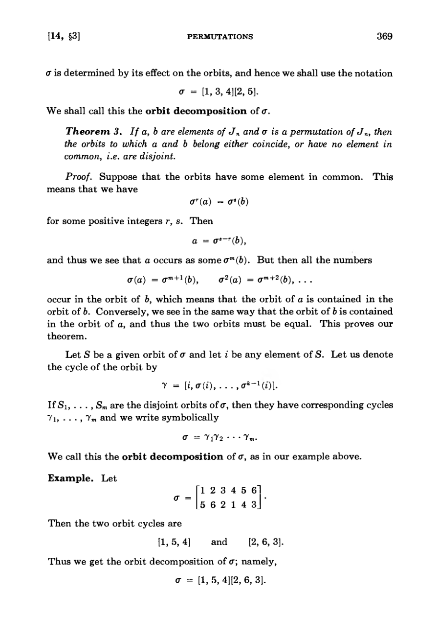
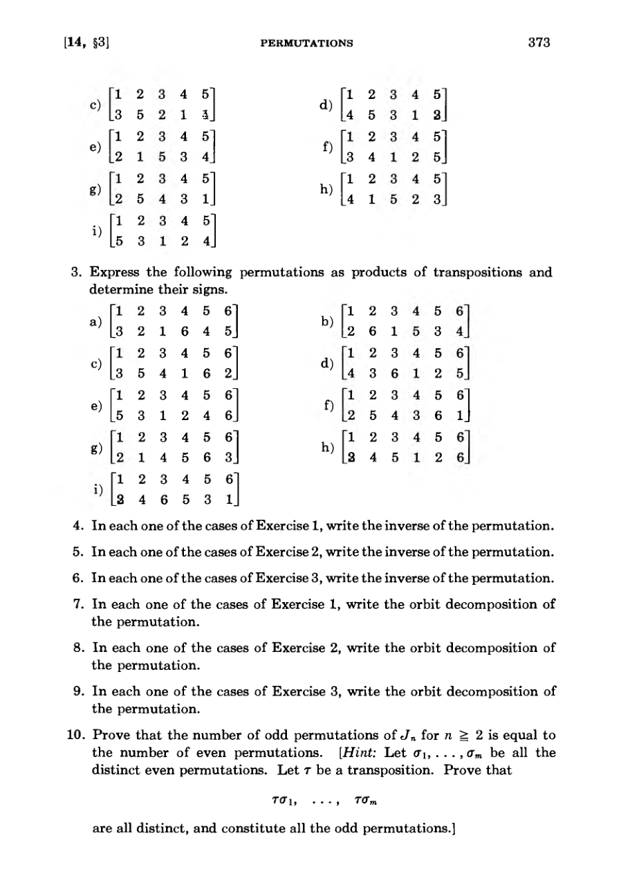
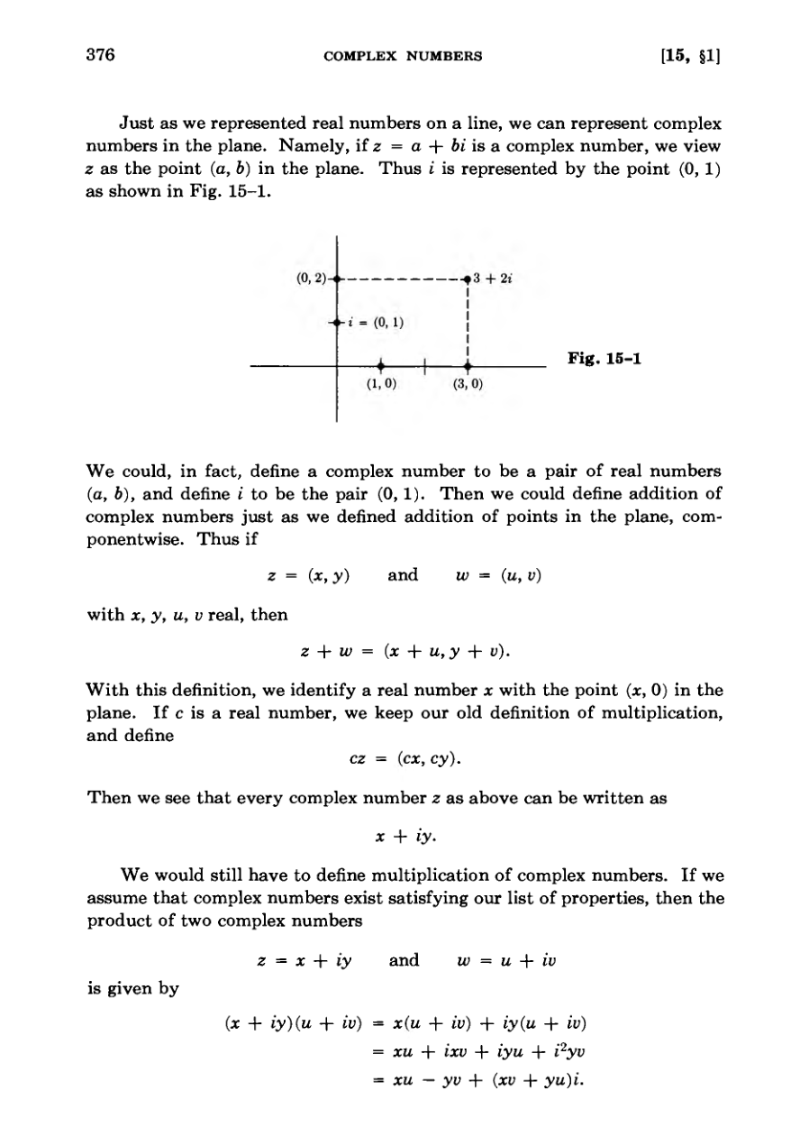
Publication details and copyright information for Serge Lang's textbook 'Basic Mathematics' (1971).
Author acknowledgments expressing appreciation to the publisher, manuscript reviewers, and exercise answer key contributors.
A detailed foreword outlining the book's intended uses in high school and college, pedagogical philosophy, and advice for students and instructors.
A comprehensive table of contents dividing the book into Algebra, Intuitive Geometry, Coordinate Geometry, and Miscellaneous mathematical topics.
Rules of Number Operations
The text develops systematic rules for operations and relations involving numbers, including addition, multiplication, and roots.
Many algebraic properties, such as commutativity and associativity, apply broadly to other mathematical objects like functions and mappings.
The primary goal is to condition the reader to have efficient reflexes in handling basic number operations.
The selection of assumed rules is designed to be foundational, simple to prove from, and widely applicable across mathematics.
The organization moves progressively through integers, rational numbers, and real numbers to demonstrate how rules hold in increasingly general contexts.
The whole first part on algebra is much more dry than the rest of the book, and it is good to motivate this algebra through geometry.
Extending Number Systems
Mathematical systems often expand to allow equations to be solved that were impossible in smaller systems.
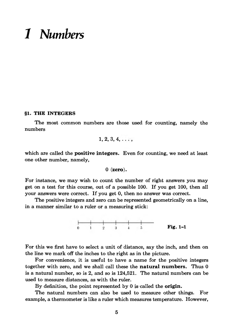
Positive integers and zero together form the natural numbers used for counting and measuring distances.
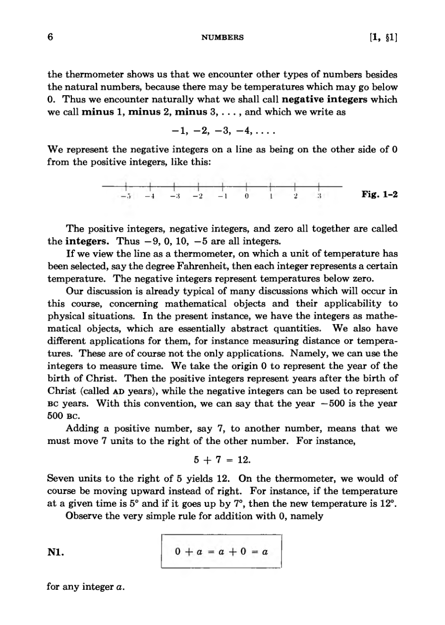
Negative integers emerge naturally when measuring phenomena that extend below zero, such as temperatures.
The combination of positive integers, negative integers, and zero constitutes the integers.
Abstract mathematical objects like integers find practical physical applications in measuring distance, temperature, and time.
This pattern is related to the extension of one system of objects to a larger system, in which more equations can be solved than in the smaller system.
DiagramDiagram
Adding Negative Numbers and Integers
Adding a negative number corresponds to moving left on the number line, just as subtraction lowers the temperature.
Every integer a has an additive inverse -a such that their sum equals zero.
The term 'minus a' is preferred over 'negative a' because -a is not necessarily negative unless a is positive.
Integer addition satisfies both the commutative property and the associative property.
Double negation yields the original number, meaning a equals minus minus a for any integer.
I find the words “negative a” confusing, because they suggest that —a is a negative number.
Diagram
Rules of Addition
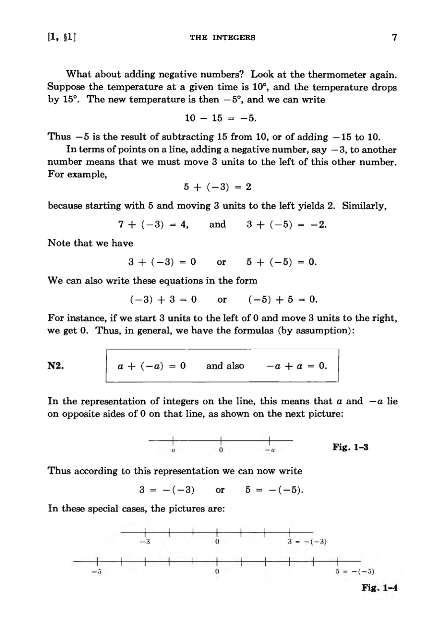
Numbers and their negatives occur symmetrically on opposite sides of zero on the number line.
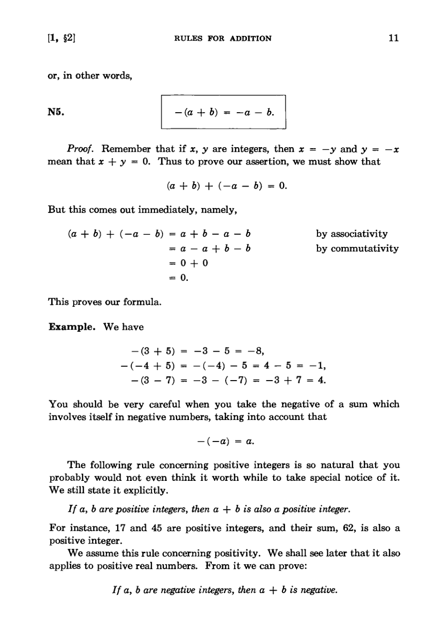
The negative of a sum equals the sum of the negatives, expressed as negative a minus b.
The sum of two positive integers is always positive, and the sum of two negative integers is always negative.
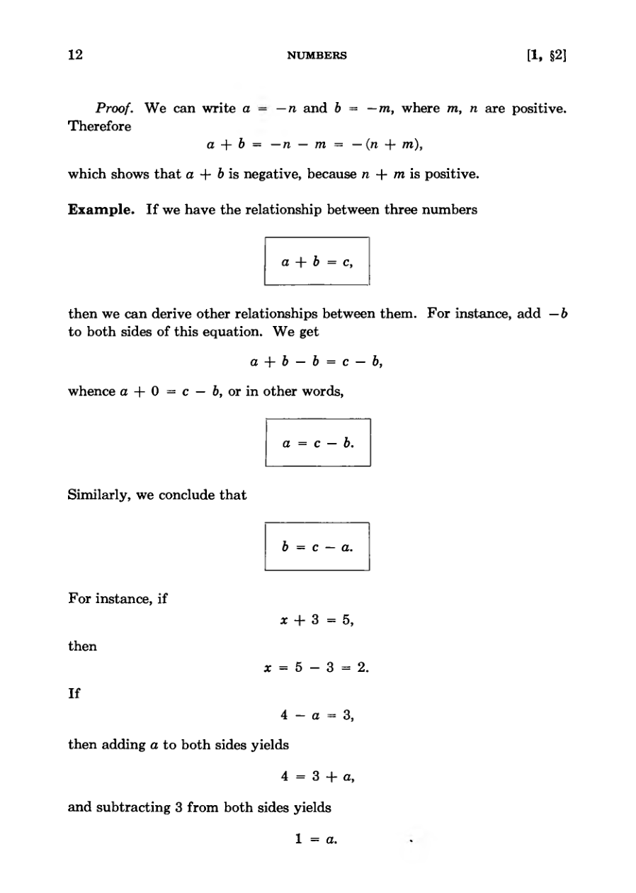
Algebraic relationships can be manipulated by adding or subtracting terms from both sides of an equation.
Rules of commutativity and associativity govern operations and allow for the proof of various arithmetic identities.
In the geometric representation of numbers on the line, a and —a occur symmetrically on the line on opposite sides of 0.
FigureDiagram
Rules for Multiplication
Multiplication rules include properties like identity, zero multiplication, commutativity, associativity, and distributivity.
Explicit numbers and literal variables can be grouped separately using algebraic properties to simplify expressions.
Fundamental rules such as right-distributivity and the zero-product rule can be logically derived from basic assumptions.
Operating with negative numbers follows rigorous laws, including the principle that the product of two negatives is a positive.
Repeated multiplication of a number by itself is conveniently abbreviated using exponential notation like a squared or cubed.
This is one of the most frequent sources of error when we work with multiplication and addition.
Diagram
Rules for Multiplication and Powers
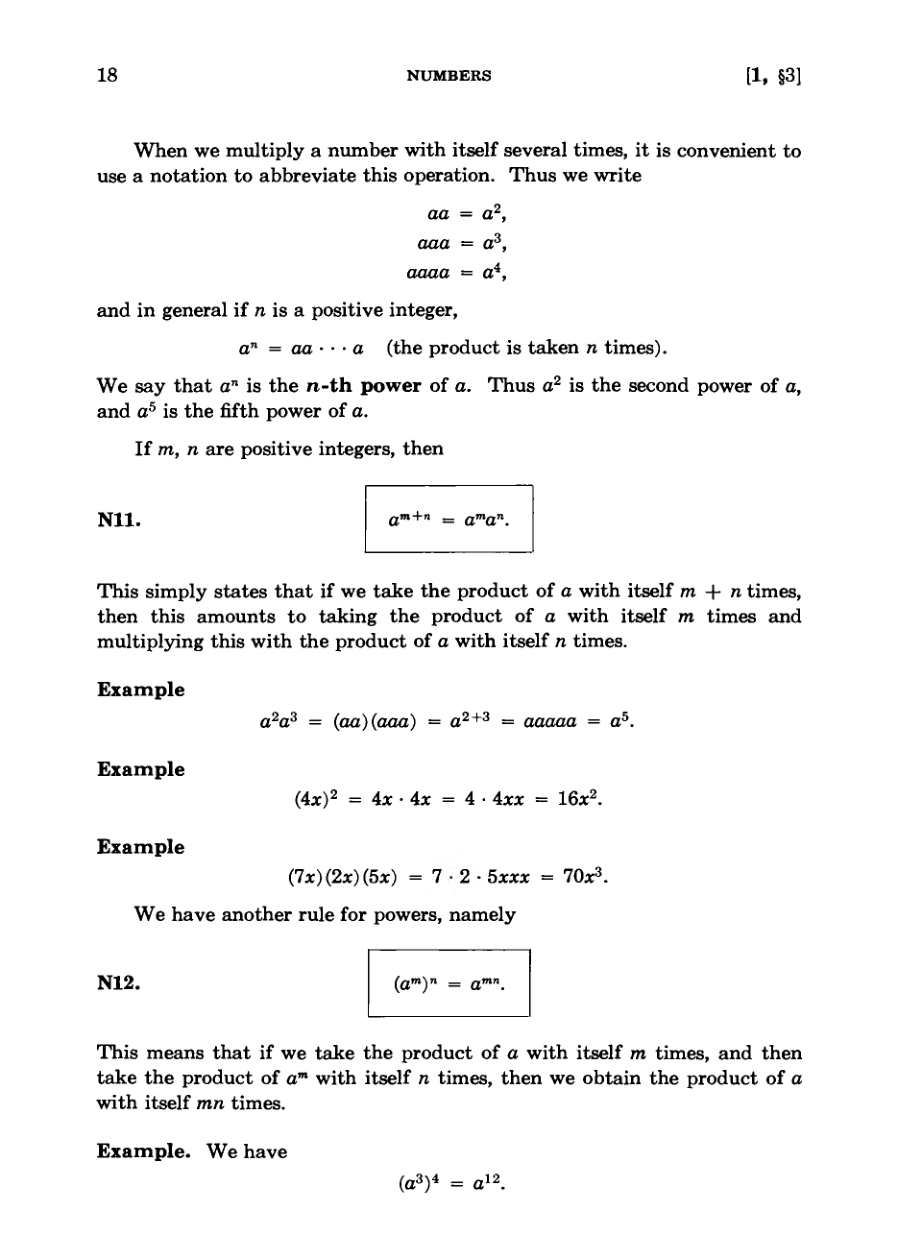
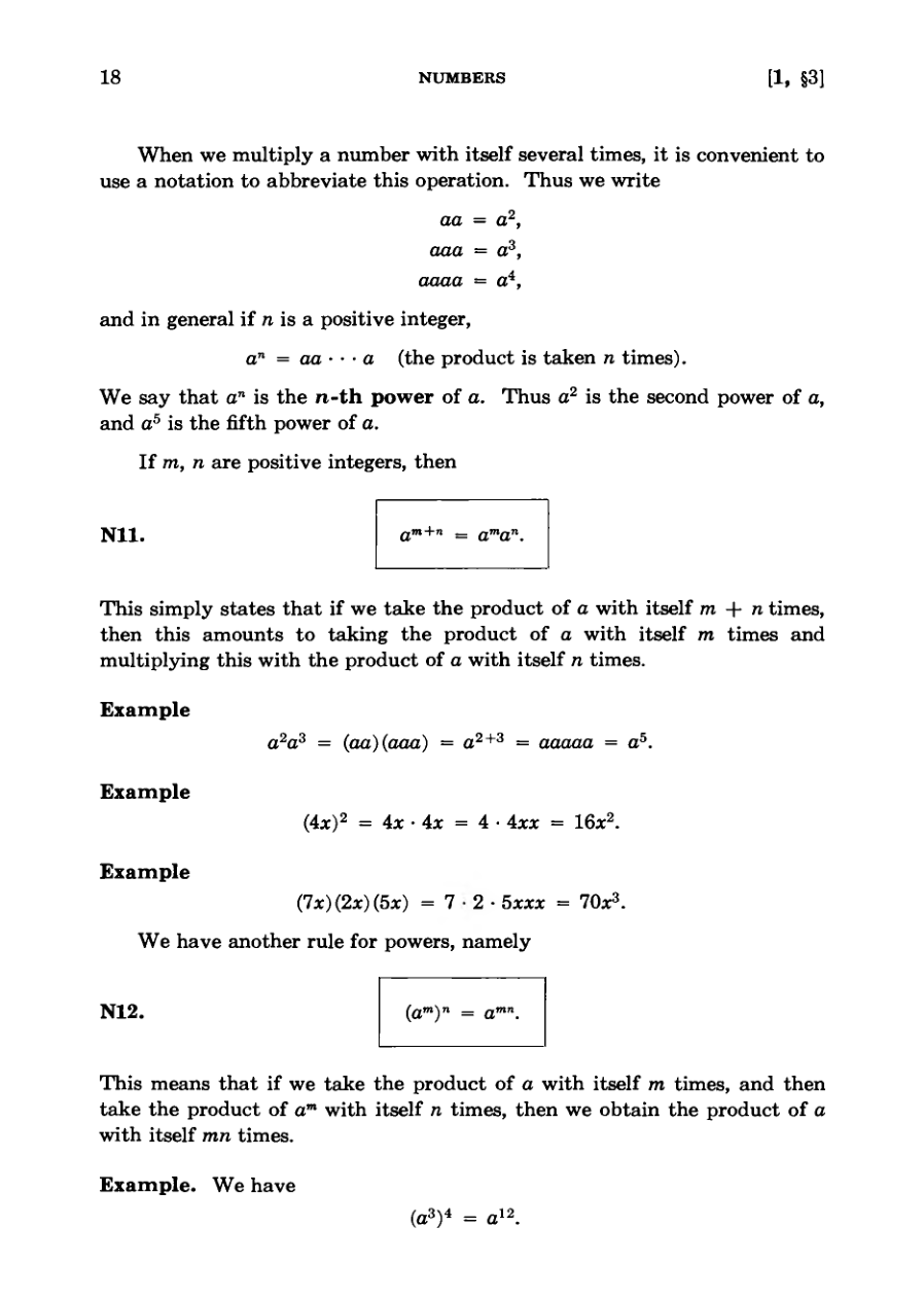
The text defines powers of numbers and variables, establishing that the product of the n-th power and m-th power of a equals the sum of their exponents.
Additional exponent rules dictate that raising a power to another power multiplies the exponents, and a product raised to a power distributes to each factor.
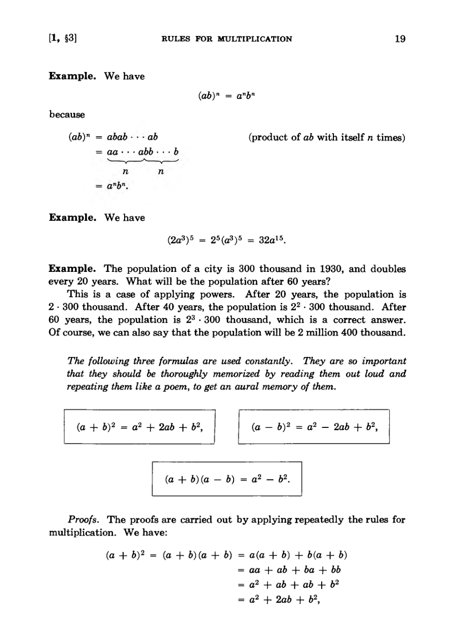
Practical applications demonstrate how these exponent rules solve real-world problems, such as calculating population growth over time.
Three fundamental algebraic formulas for squaring binomials and finding the difference of squares are introduced and proven using multiplication rules.
Step-by-step examples illustrate the expansion of binomials and polynomials by systematically applying distribution and combining like terms.
They are so important that they should be thoroughly memorized by reading them out loud and repeating them like a poem to get an aural memory of them.
DiagramDiagram
Even and Odd Integers
The text provides algebraic practice problems involving polynomial multiplication and exponential population growth word problems.
Positive integers are divided into two fundamental categories: odd integers and even integers.
An even integer can be expressed algebraically in the form 2n, while an odd integer can be written as 2n + 1 or 2m - 1.
Basic arithmetic theorems dictate how the sums of even and odd numbers behave, demonstrating that the sum of an even and an odd number is always odd.
Proofs are provided to show that the square of an even integer is even and the square of an odd integer is odd.
Thus the odd integers go up by 2 and the even integers go up by 2.
Divisibility and Rational Numbers
Even and odd integers provide a foundation for understanding divisibility, where an integer d divides n if m equals dk for some integer k.
Every integer is divisible by one and every positive integer is divisible by itself.
Exercises challenge students to prove various algebraic properties of even and odd numbers, powers, and modulo arithmetic.
Rational numbers are defined as ordinary fractions or quotients of integers where the denominator cannot be zero.
Fractions lack a unique representation, leading to the rule of cross-multiplying to determine when two expressions yield the same rational number.
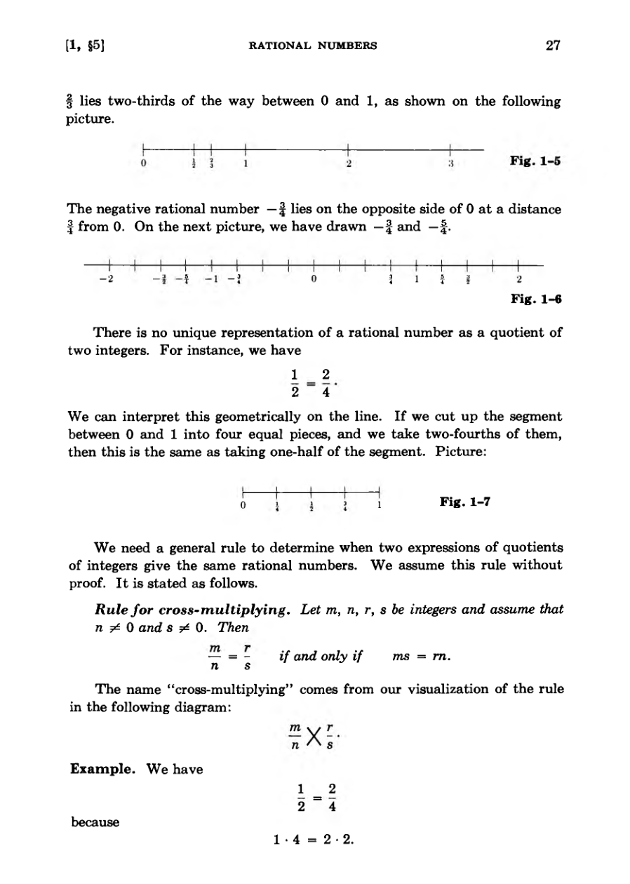
There is no unique representation of a rational number as a quotient of two integers.
Diagram
Rational Numbers and Cancellation
Integers can be treated as rational numbers by expressing them over one, such as m equals m over one.
Cross-multiplication applies to both positive and negative integers and forms the foundation for testing equality in fractions.
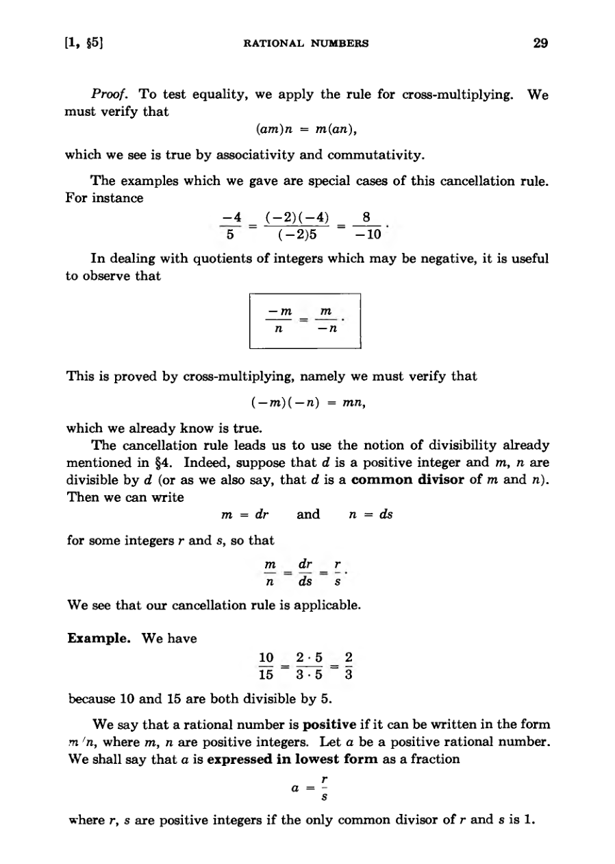
The cancellation rule demonstrates that multiplying or dividing the numerator and denominator by the same non-zero integer preserves the fraction's value.
Divisibility and greatest common divisors allow fractions to be simplified into a lowest form.
Every positive rational number is guaranteed to have a simplified expression in lowest form where the numerator and denominator share no common divisors other than one.
Some people view this proof as the reason why cross-multiplication works.
Diagram
Adding and Multiplying Fractions
Rational numbers are expressed as quotients of integers and can be adjusted to share a common denominator.
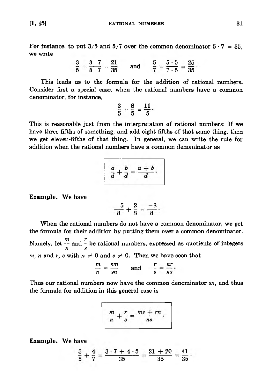
The addition of rational numbers with a common denominator is derived naturally from the meaning of fractions.
Fractions with different denominators are added by first converting them to a shared common denominator.
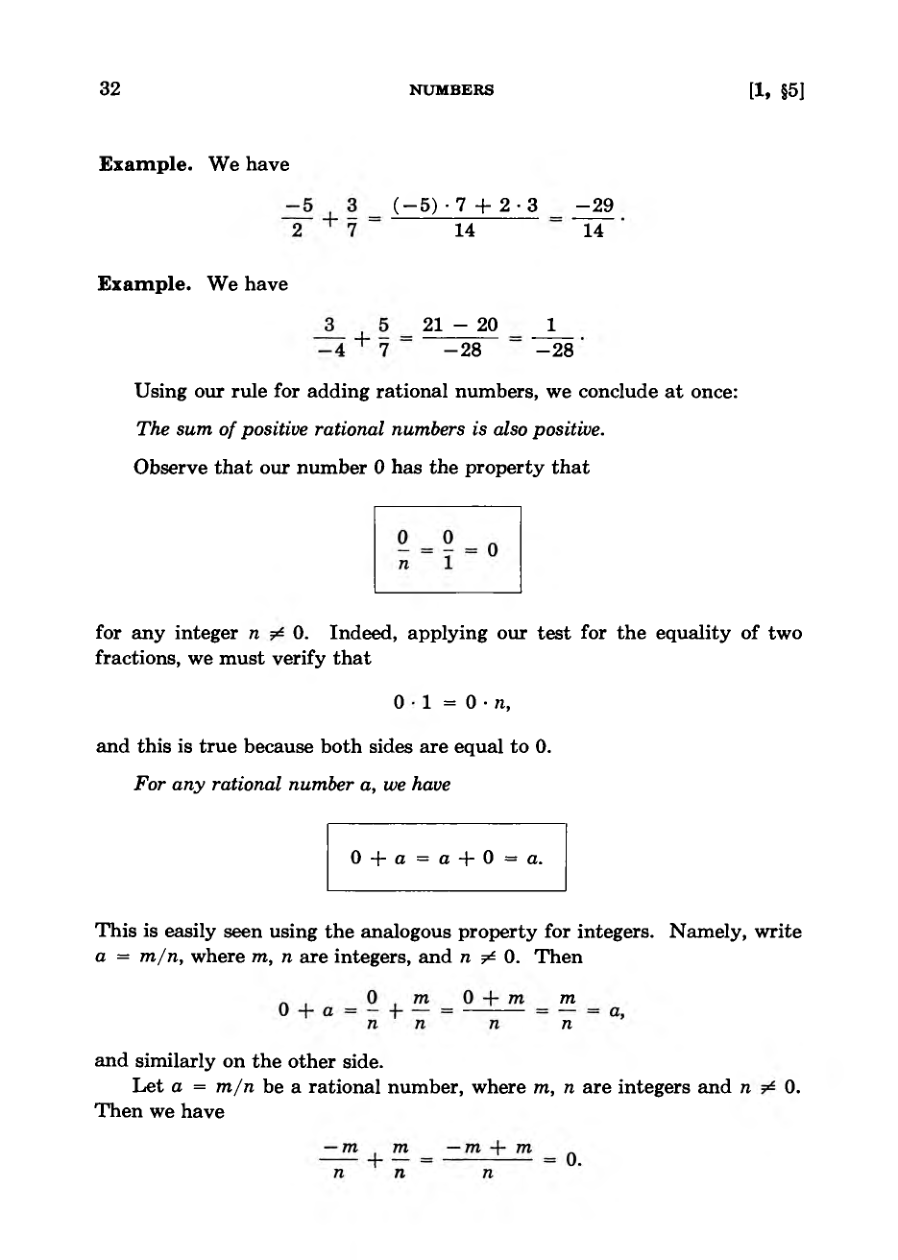
The sum of positive rational numbers remains positive, and the number zero acts as an additive identity.
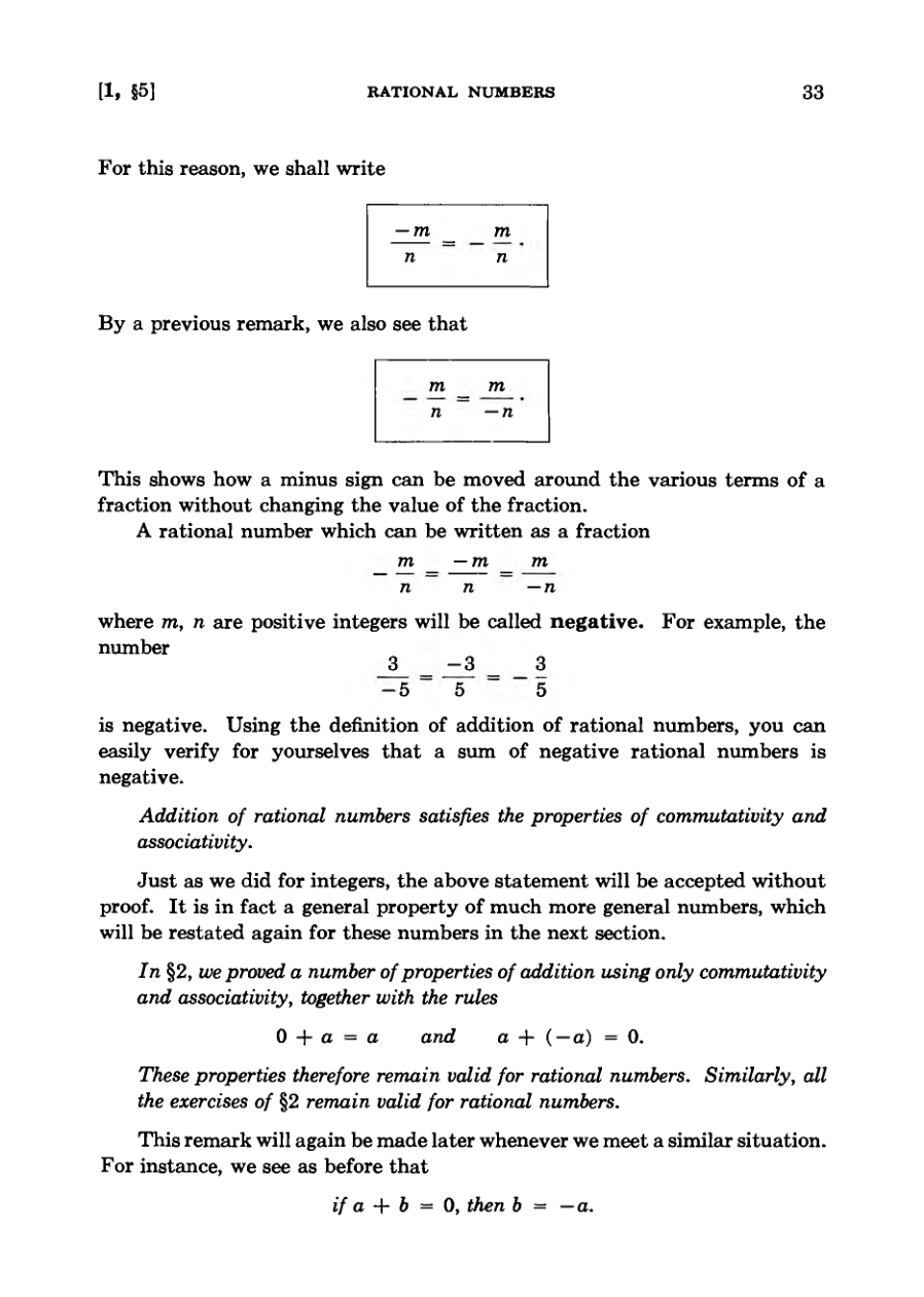
Negative rational numbers are defined using the placement of minus signs, and their sums behave predictably.
Addition of rational numbers follows the properties of commutativity and associativity, extending previous rules established for integers.
If we have three-fifths of something, and add eight-fifths of that same thing, then we get eleven-fifths of that thing.
DiagramDiagramDiagramDiagram
Multiplying Fractions and Square Roots
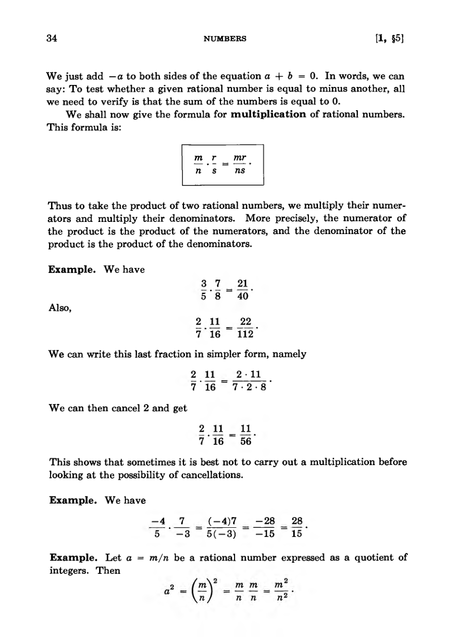
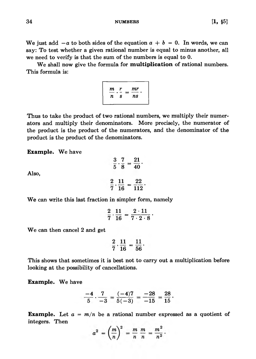
Fractions are multiplied by multiplying their numerators together and their denominators together.
Simplifying fractions before completing multiplications can prevent unnecessary computational complexity.
Real-world problems, such as radioactive decay or substance disintegration, can be modeled using fraction multiplication.
Systematic decimal approximation methods can be used to search for the square root of 2.
Despite getting arbitrarily close through approximations, a rigorous mathematical theorem proves that no positive rational number actually has a square of 2.
However, to find a rational number whose square is 2, the procedure is a bummer because of the following theorem.
Diagram
Rational Numbers and Equations
The proof that the square root of two is irrational concludes by showing that an original assumption leads to a contradiction.
Multiplication of rational numbers follows the same basic rules and algebraic formulas as integers.
Linear equations with rational numbers can be solved using standard algebraic manipulations like distribution and isolation of variables.
Fractions and algebraic steps can be handled in multiple valid ways to arrive at the correct solution.
The section concludes with a comprehensive set of exercises covering equation solving, fractions, and factorials.
Thus from our original assumption that (m/n)2 = 2 and m/n is in lowest form, we have obtained the impossible fact that both m, n are even.
Rational Numbers and Multiplicative Inverses
Exercises challenge students to prove the non-existence of certain positive rational roots for numbers like two, three, and five.
Decimal approximation problems require finding rational numbers whose squares or cubes approach specific roots to various degrees of accuracy.
Word problems involving chemical decay, bacterial populations, and lake pollution illustrate exponential decrease and fractions of remaining substances over time.
Population growth problems demonstrate how city sizes change incrementally over multi-year periods.
The text introduces multiplicative inverses for non-zero rational numbers, defining them such that a multiplied by its inverse equals one.
Mathematical proofs use the existence of multiplicative inverses to deduce that if the product of two numbers is zero, at least one of the numbers must be zero.
A chemical substance decomposes in such a way that it halves every 3 min.
Rational Numbers and Fractions
The text extends the rules of quotients and cross-multiplication from integers to rational numbers.
Cross-multiplication states that if a/b = c/d, then ad = bc, and vice versa, proven using basic field properties.
The cancellation law for multiplication allows one to deduce b = c from ab = ac provided a is non-zero.
Fractions involving rational numbers can be manipulated using common denominators and standard addition formulas.
Algebraic equations containing rational expressions can be solved systematically by applying cross-multiplication.
Thus we can operate with fractions formed with rational numbers much as we could operate with fractions formed with integers.
Algebraic Word Problems and Proofs
The fundamental physics formula relating distance, speed, and time is introduced as d = st.
Practical applications are demonstrated through word problems involving travel speed and mixture concentrations.
Linear equations are formulated with single variables to solve real-world scenarios such as driving times and antifreeze replacement.
Exercises are provided to test algebraic manipulation, equation solving, and relation proofs.
Advanced exercises challenge students to prove various polynomial and rational expressions using cross-multiplication.
A person takes a trip and drives 8 hr, a distance of 400 mi.
Solving Linear Equations
A collection of word problems covers temperature conversions, electrical resistance, mixture concentrations, and travel times.
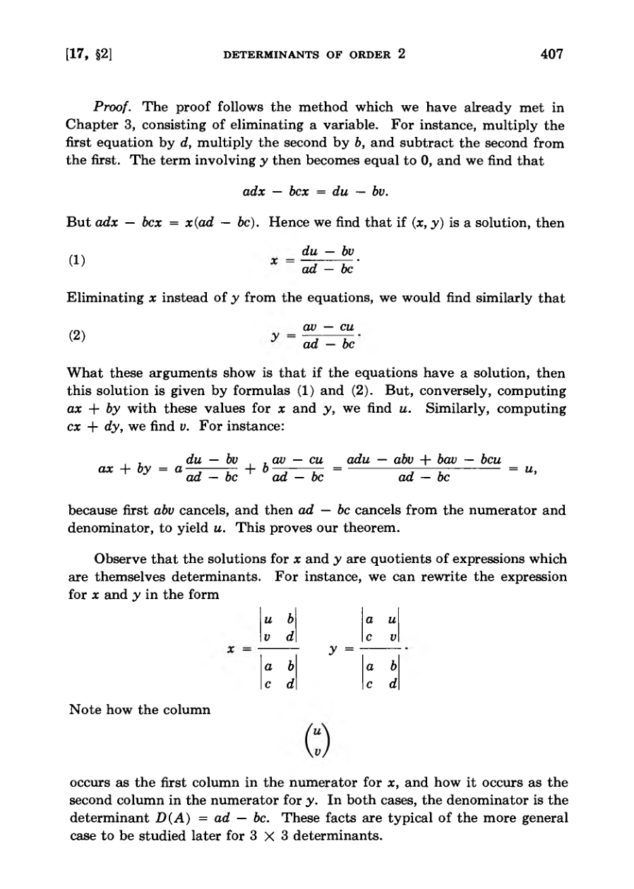
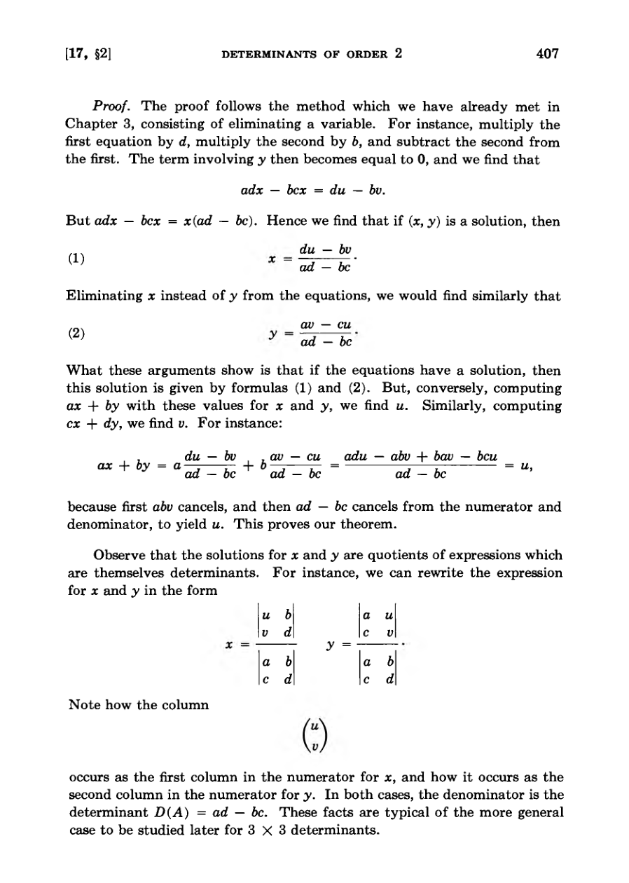
The text introduces systems of two linear equations with two unknowns.
The elimination method is demonstrated by multiplying equations to make coefficients of one variable match.
Subtracting or adding the manipulated equations successfully cancels out one variable to solve for the other.
Substitution is then used to find the value of the remaining variable, completing the solution set.
We try to get rid of x, say, so as to obtain only one equation in y.
Solving Linear Equations
Some linear equation systems lack solutions when the equations represent parallel lines.
Solutions usually exist for simple systems of two equations in two unknowns.
Simultaneous equations correspond to finding the intersection point of straight lines in coordinate geometry.
The elimination procedure guarantees valid solutions that can be checked explicitly.
Word problems involving distance and speed can be effectively solved using two variables.
We don’t intend to overburden you or give you any worries about them.
Solving Linear Equations
Systems of two linear equations can be solved to find specific values for variables like x and y.
Equations with three unknowns are solved by systematically eliminating variables one by one.
Strategic ordering of equations during elimination makes the algebraic process significantly easier.
Back-substitution allows us to find the remaining variable values once one variable is known.
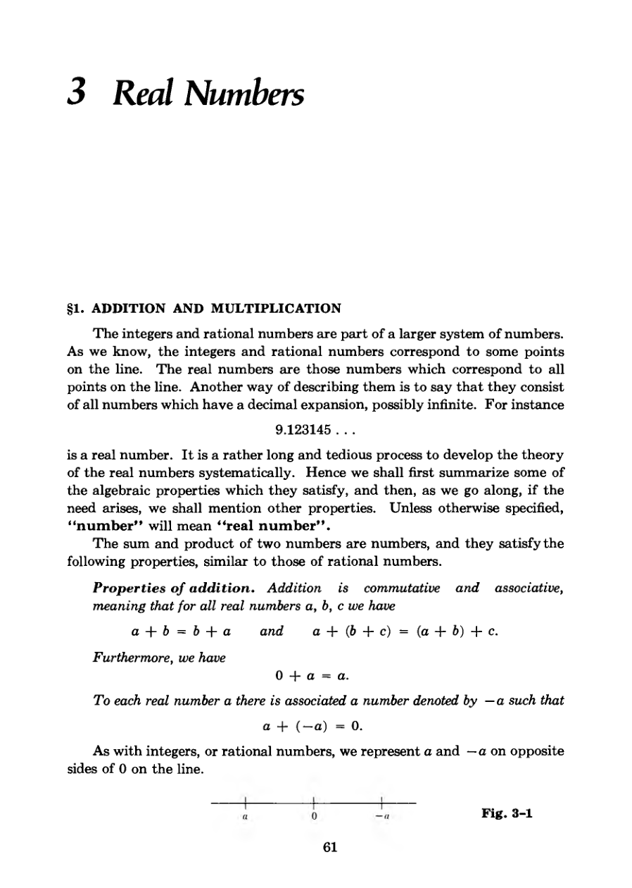
The chapter introduces real numbers as corresponding to all points on a line with decimal expansions.
We choose the order of elimination so as to make it easier on ourselves.
Diagram
Real Numbers Properties and Positivity
Every real number has a unique additive inverse represented as negative a.
Multiplication of real numbers is commutative, associative, and distributive over addition.
Real numbers share the same basic algebraic properties as integers and rational numbers.
Every non-zero real number possesses a unique multiplicative inverse, denoted as one over a.
Systems with only two objects, such as even and odd abstractions, can satisfy these same basic arithmetic properties.
Positivity is defined by specific foundational rules where the product and sum of positive numbers remain positive.
Thus real numbers are not the only system to satisfy these properties.
DiagramDiagram
Positivity and Square Roots
Basic rules of positivity establish properties for products and reciprocals of positive and negative real numbers.
Every positive real number is assumed to have a square root, proving the existence of irrational numbers like the square root of two.
Algebraic factoring demonstrates that any positive number has precisely two square roots, one positive and one negative.
Mathematical convention designates the unique positive square root with the radical symbol while the other is its negative counterpart.
The principal square root of a squared number introduces the definition of absolute value as a non-negative quantity.
Because of this, and Theorem 4, §5 of Chapter 1, we now see that a number whose square is 2 is irrational, but exists as a real number.
Rationalizing Square Roots
The process of removing square roots from either the numerator or the denominator is achieved using the algebraic rule for the difference of squares.
While eliminating roots from the denominator is often taught as a standard technique, having a square root in the denominator is frequently useful in practice.
Advanced calculus techniques often require rationalizing the numerator to transform expressions into more workable forms.
Both rationalizing procedures rely on multiplying both the numerator and denominator by a conjugate expression.
These algebraic manipulations are essential preparation for upcoming topics such as the Pythagorean Theorem and calculating distances.
This example has the same notation as an actual case which arises in more advanced courses of calculus.
Powers and Roots
Exercises involving absolute value equations and rationalizing expressions precede the formal introduction of powers and roots.
The n-th root of a positive real number is defined as the unique positive real number r whose n-th power equals a.
Fractional powers extend the concept of exponents to rational numbers while preserving fundamental algebraic rules.
Zero and negative exponents are naturally derived, showing that a to the power of zero is one and negative powers represent multiplicative inverses.
Rational exponents can be decomposed into a combination of integer powers and n-th roots.
Let a be a positive number and let n be a positive integer. As part of the properties of real numbers, we assume, but do not prove, that there exists a unique positive real number r such that rn = a.
Diagram
Real Numbers and Inequalities
Real numbers are distinguished from rational numbers by the existence of numbers like square roots and general exponents.
Elementary calculus courses often assume the existence of certain real numbers and postpone formal proofs to advanced courses.
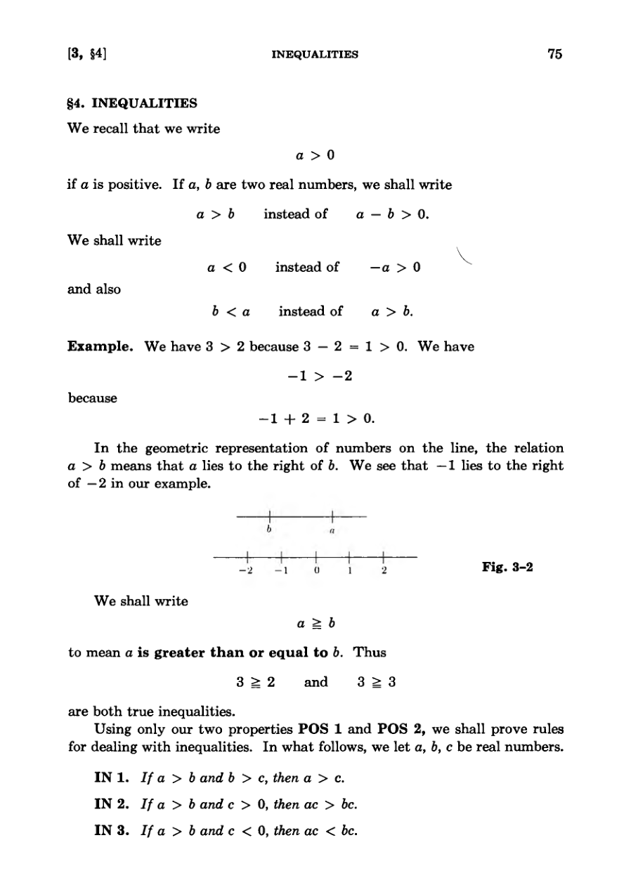
Inequalities are defined formally using positivity, where a > b means that a - b > 0.
Multiplying both sides of an inequality by a positive number preserves the inequality.
Multiplying both sides of an inequality by a negative number reverses the direction of the inequality.
Rule IN 3 tells us that if we multiply both sides of an inequality by a negative number, then the inequality gets reversed.
Diagram
Proving Inequalities and Intervals
Basic properties of inequalities, such as IN 2, are proved systematically using foundational rules.
Linear inequalities like 2x - 4 > 5 are solved by finding equivalent simpler conditions.
Solving inequalities with variables in the denominator requires splitting the domain into separate cases.
Rational inequalities may lead to impossible conditions, eliminating certain cases from the solution set.
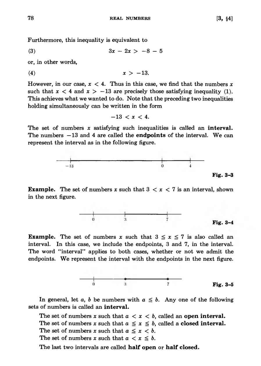
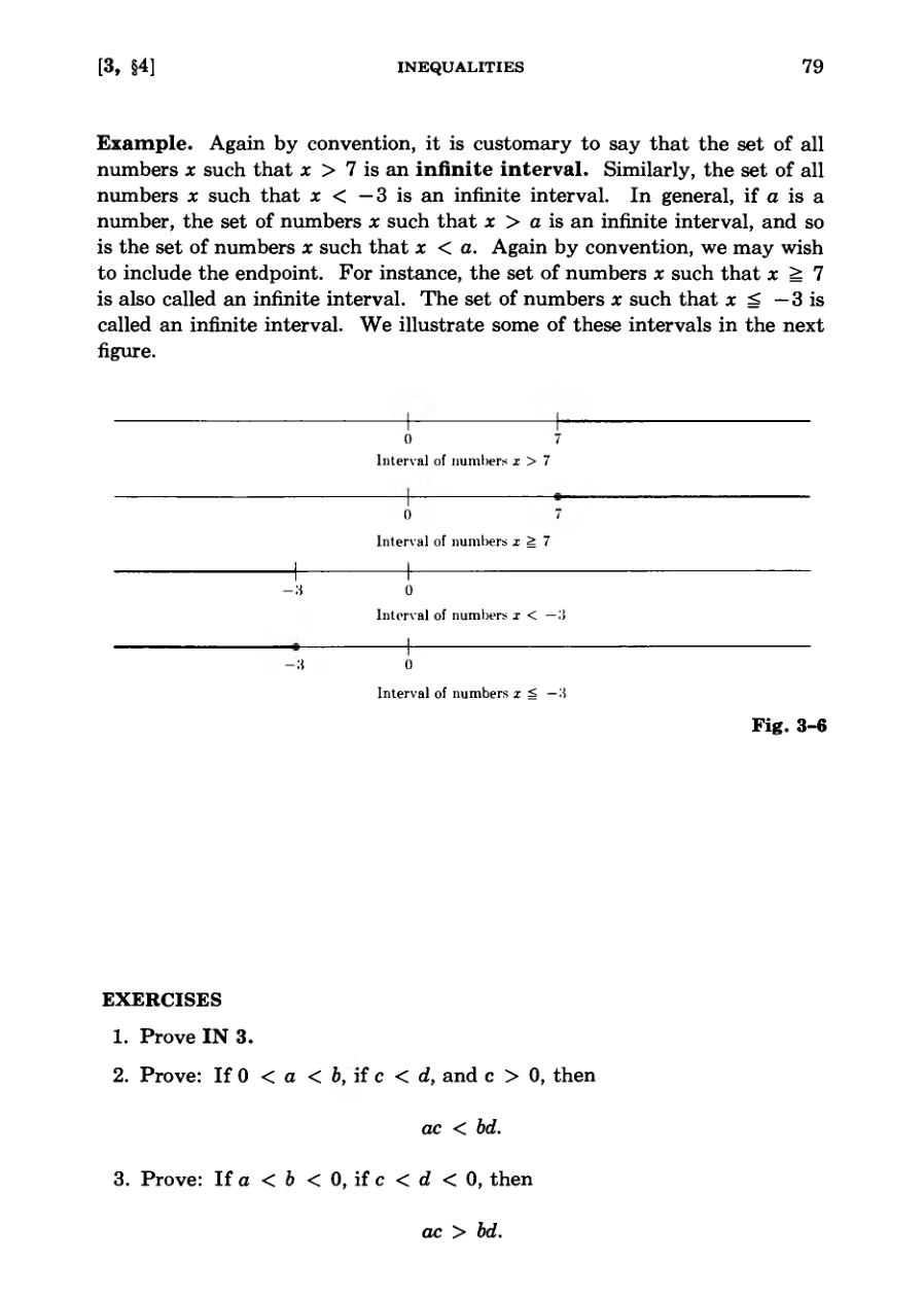
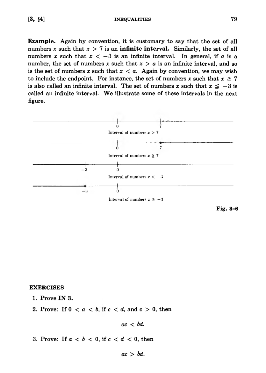
Combinations of inequalities define bounded or infinite intervals, categorized as open, closed, or half-open.
Note that the quotient on the left makes no sense if x = 4.
DiagramDiagram
Real Numbers and Quadratic Equations
A series of mathematical exercises challenge the reader to prove fundamental properties of inequalities and real numbers.
The text introduces the concept of mathematical induction to formalize stepwise proofs for powers of inequalities.
Exercises also require solving numerous linear inequalities and finding intervals for variable x.
The chapter transitions to quadratic equations, moving beyond linear equations where x appears only in the first power.
Completing the square is demonstrated as a core method to solve quadratic equations and derive general formulas.
Examples illustrate that some quadratic equations yield multiple real solutions while others have no solutions in real numbers.
But a negative real number cannot possibly be a square of a real number and we conclude that our equation does not have a solution in real numbers
Diagram
Deriving The Quadratic Formula
Equations with a coefficient on the squared term can be simplified by dividing the entire equation by that coefficient.
Completing the square on a general quadratic equation yields the general quadratic formula.
The discriminant determines whether an equation has two solutions, one solution, or no real solutions.
If the discriminant is negative, the equation has no solution within the real numbers.
The quadratic formula should be memorized thoroughly, even by reading it aloud like a poem.
Extending real numbers to a larger system allows for taking square roots of negative numbers, making the formula universally valid.
Read it out loud like a poem, to get an aural memory of it: “x equals minus b plus or minus square root of b squared minus four ac over two a.”
On Reading Mathematics Books
The text provides a series of quadratic equations to solve using formulas and extended number systems.
It transitions into an interlude discussing different methods for reading mathematical texts.
Books must be organized linearly on pages, which distorts the natural simultaneity of how the human brain perceives ideas.
Readers are encouraged to start in the middle, skip ahead, or skim rather than strictly reading from beginning to end.
Logical proof is defined as a sequence of statements built upon assumptions and common-sense rules of deduction.
In writing the book, the whole subject has to be organized in a totally ordered way, along lines and pages, which is not the way our brain works naturally.
Mathematical Logic and Converse Statements
The converse of a conditional statement interchanges its hypothesis and conclusion.
Biconditional statements combine both a conditional statement and its converse using the phrase if and only if.
The phrase only if is avoided independently because natural language tends to misinterpret its direction.
Proof by contradiction establishes the truth of a statement by showing that its negation leads to an absurdity.
Mathematical expressions require proper context and quantification to be meaningful rather than ambiguous.
Clear mathematical writing relies on the construction of complete sentences.
We want to prove that a certain statement A is true.
Mathematical Language and Sets
Incomplete mathematical symbols require proper qualifications to determine their truth value.
Equality strictly means that two expressions refer to the exact same object.
Assertions are equivalent when one is true if and only if the other is true.
Mathematical objects are distinct from their physical counterparts and operate on logical levels.
A collection of objects forms a set, and subsets describe collections where every element belongs to another set.
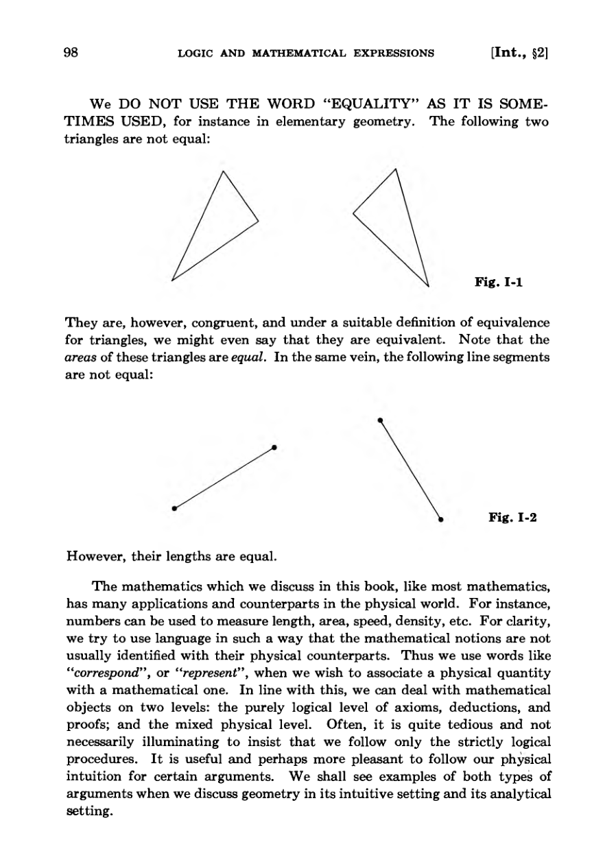
We DO NOT USE THE WORD “ EQUALITY” AS IT IS SOMETIMES USED, for instance in elementary geometry.
Diagram
Mathematical Notation and Sets
A set with no elements is defined as an empty set, such as when numerical conditions contradict each other.
Proving the equality of two sets often involves showing that each is a subset of the other.
Mathematical conventions allow variables like x and y to be equal unless explicitly stated otherwise as distinct.
Subscripts and indices are introduced to manage sequences of numbers efficiently when the alphabet runs short.
Finite sequences associate specific objects or numbers to integers within a defined range from 1 to n.
It is clear that we would soon run out of letters of the alphabet in enumerating numbers just with letters, and hence we use a notation with subscripts...
Mathematical Notation and Intuitive Geometry
Conventions for mathematical notation use specific letter types to denote numbers, points, angles, and functions consistently.
While notation should be clear, authors must navigate a limited alphabet and occasional imperfections by encouraging active learning.
Intuitive geometry in the plane is refocused on the Pythagoras theorem and congruence rather than complicated classical constructions.
Starting with the Pythagoras theorem and isometries simplifies proofs and provides a natural introduction to advanced mathematics and mappings.
The upcoming sections will transition from geometric proofs based on intuition to analytic proofs based purely on the properties of real numbers.
If you find any such things in the present book, then correct them or improve them for yourself, or write your own book.
Analytic Foundations of Geometry
Providing analytic foundations for geometry introduces powerful computational methods that intuition alone cannot easily achieve.
Mixing geometric intuition with analytic techniques yields a deeper and more comprehensive understanding of mathematical subjects.
Historical progress in mathematics was long hindered by an unnecessary inhibition against applying numbers to geometric objects.
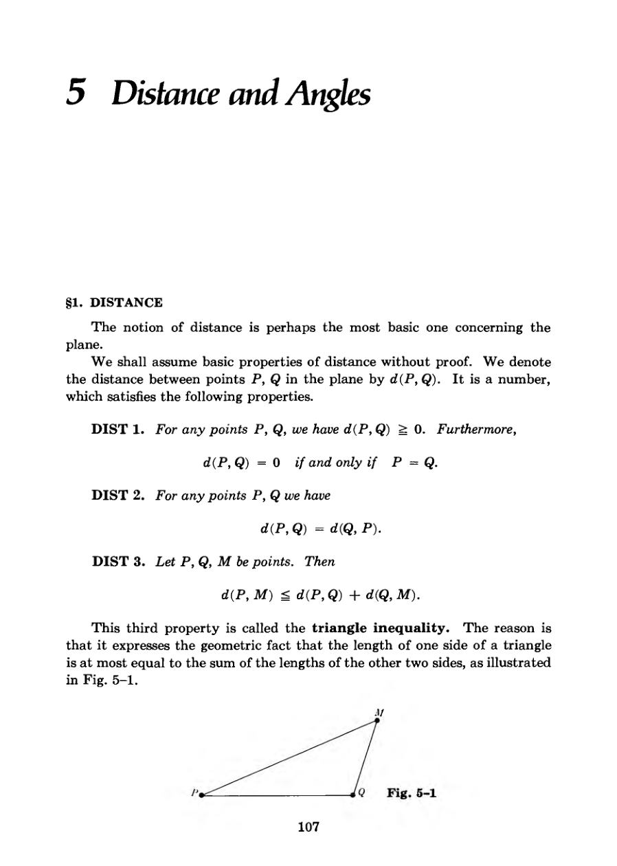
Distance in the plane is formalized through fundamental properties, including non-negativity, symmetry, and the triangle inequality.
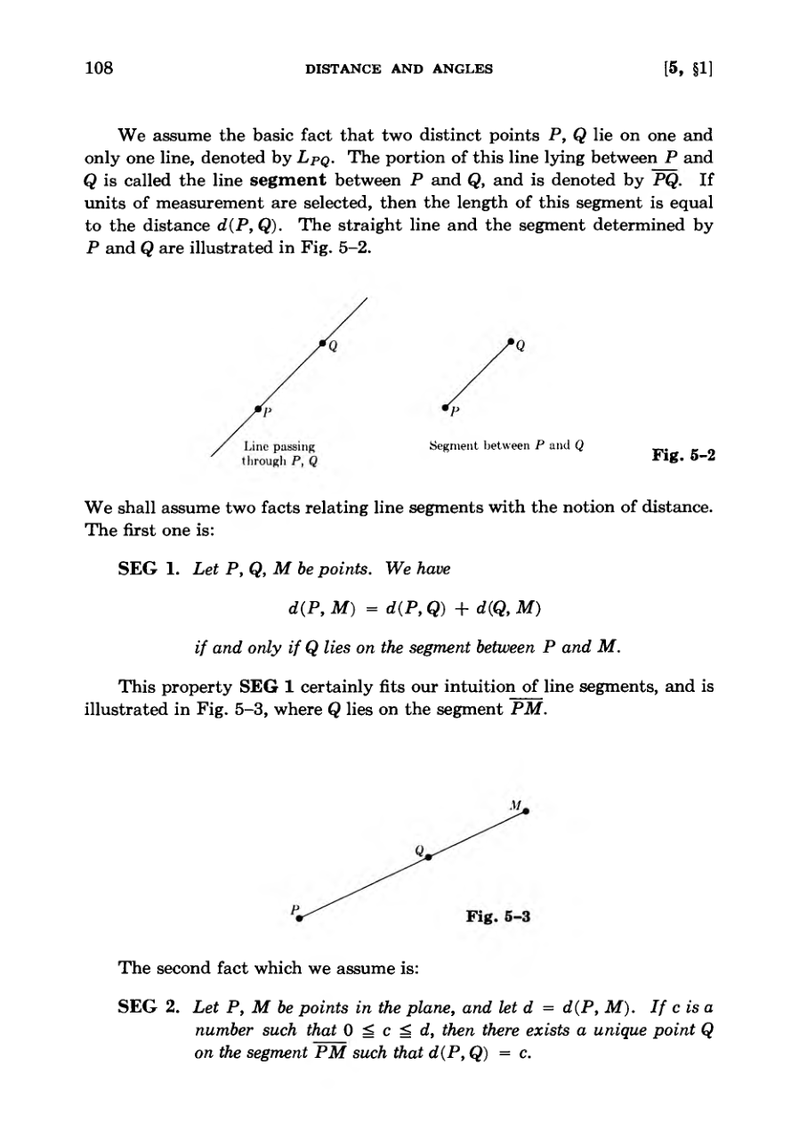
Line segments and their lengths are rigorously connected to distance functions and axiomatic properties.
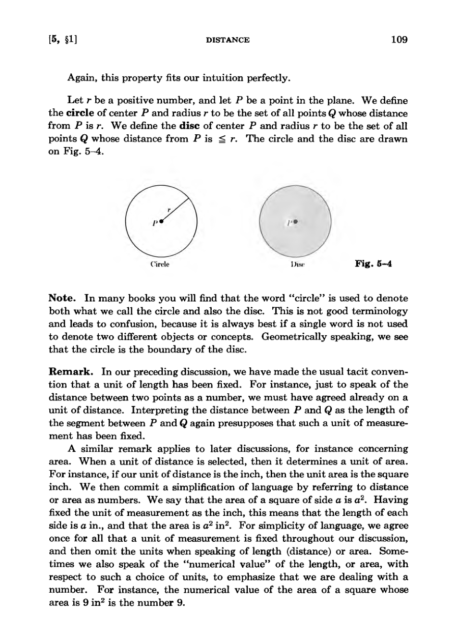
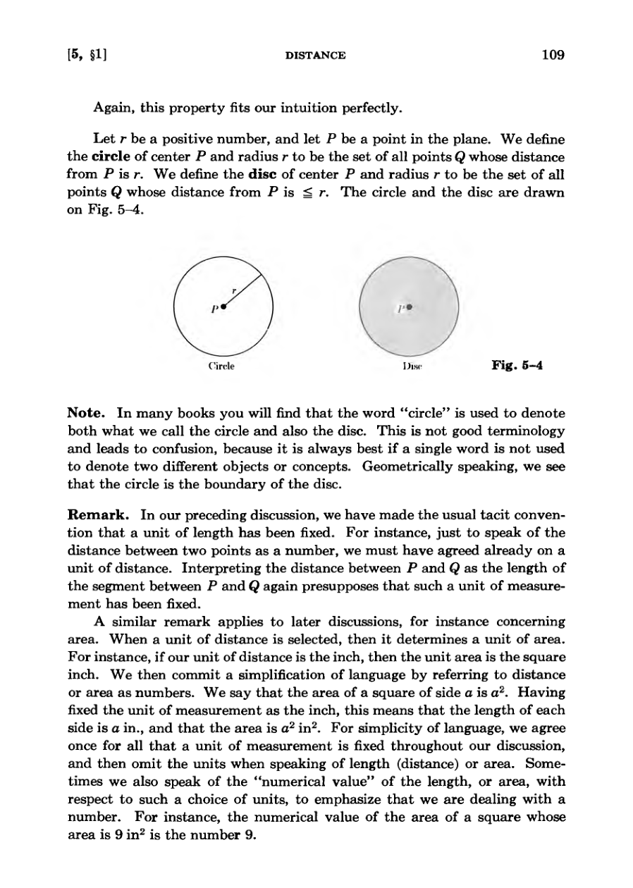
Circles and discs are carefully distinguished to avoid the terminological confusion found in many mathematical texts.
One reason why the Greeks did not get further in their mathematics is that they suffered from the inhibition of using numbers to deal with geometric objects.
DiagramDiagramFigure
Foundations of Geometric Measurement
A circle serves as the geometric boundary of a disc.
Geometric discussions require a pre-fixed unit of length and area, though units are often omitted for linguistic simplicity.
The text establishes foundational axioms regarding straight lines, parallelism, and perpendicularity in a plane.
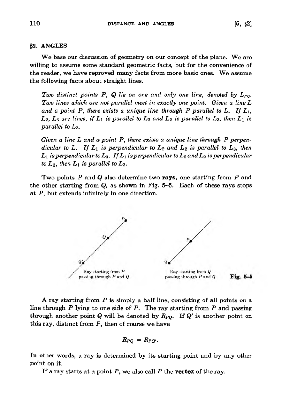
Rays are defined by a starting vertex and another point, effectively acting as half-lines extending infinitely.
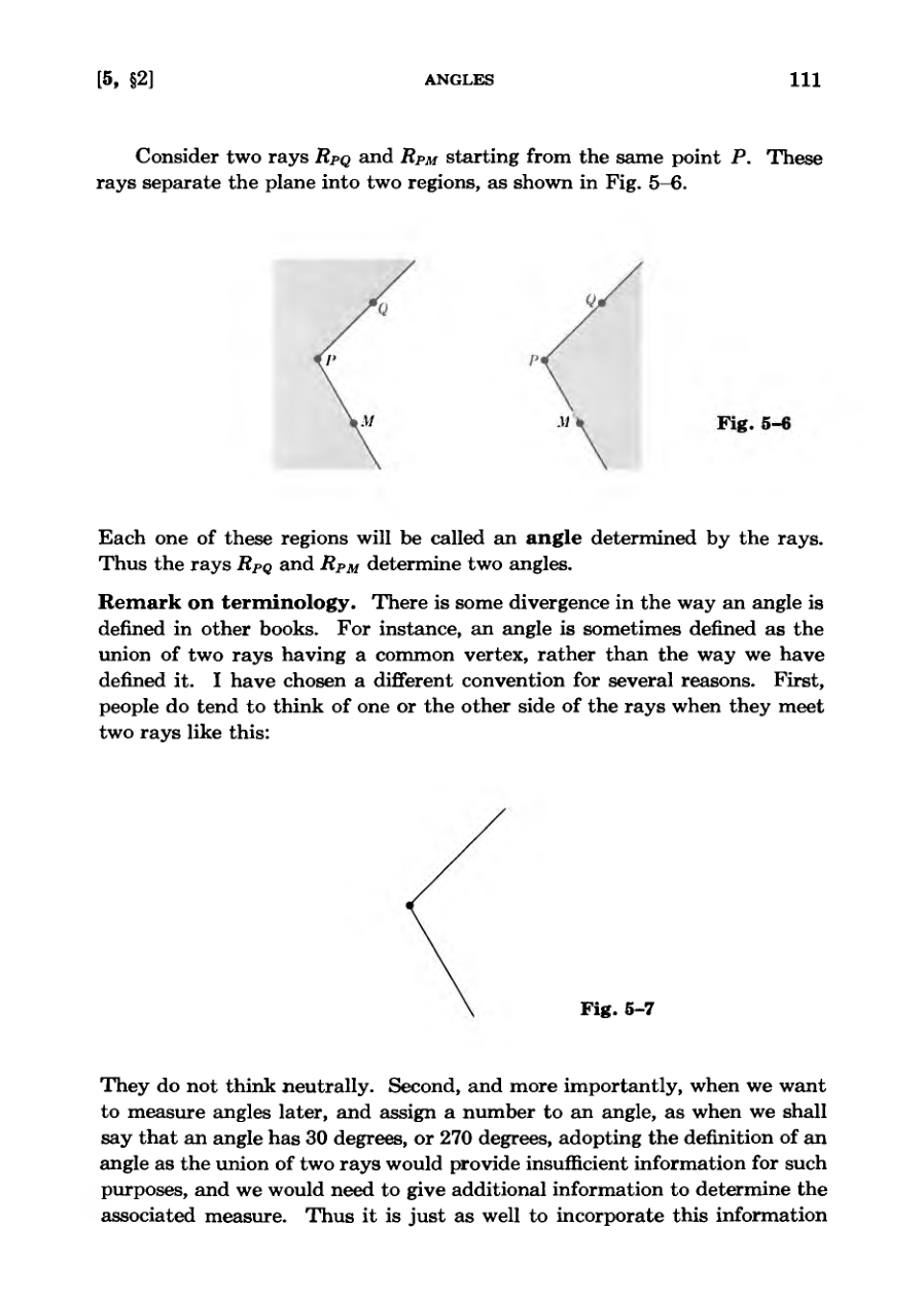
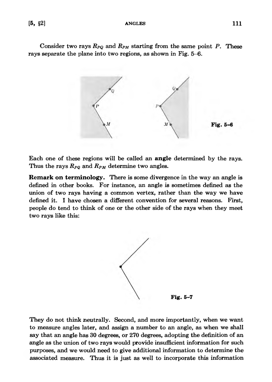
Angles are defined as regions of the plane separated by two rays sharing a common vertex rather than simply the union of the rays.
They do not think neutrally.
FigureDiagramDiagram
Defining Angles and Arcs
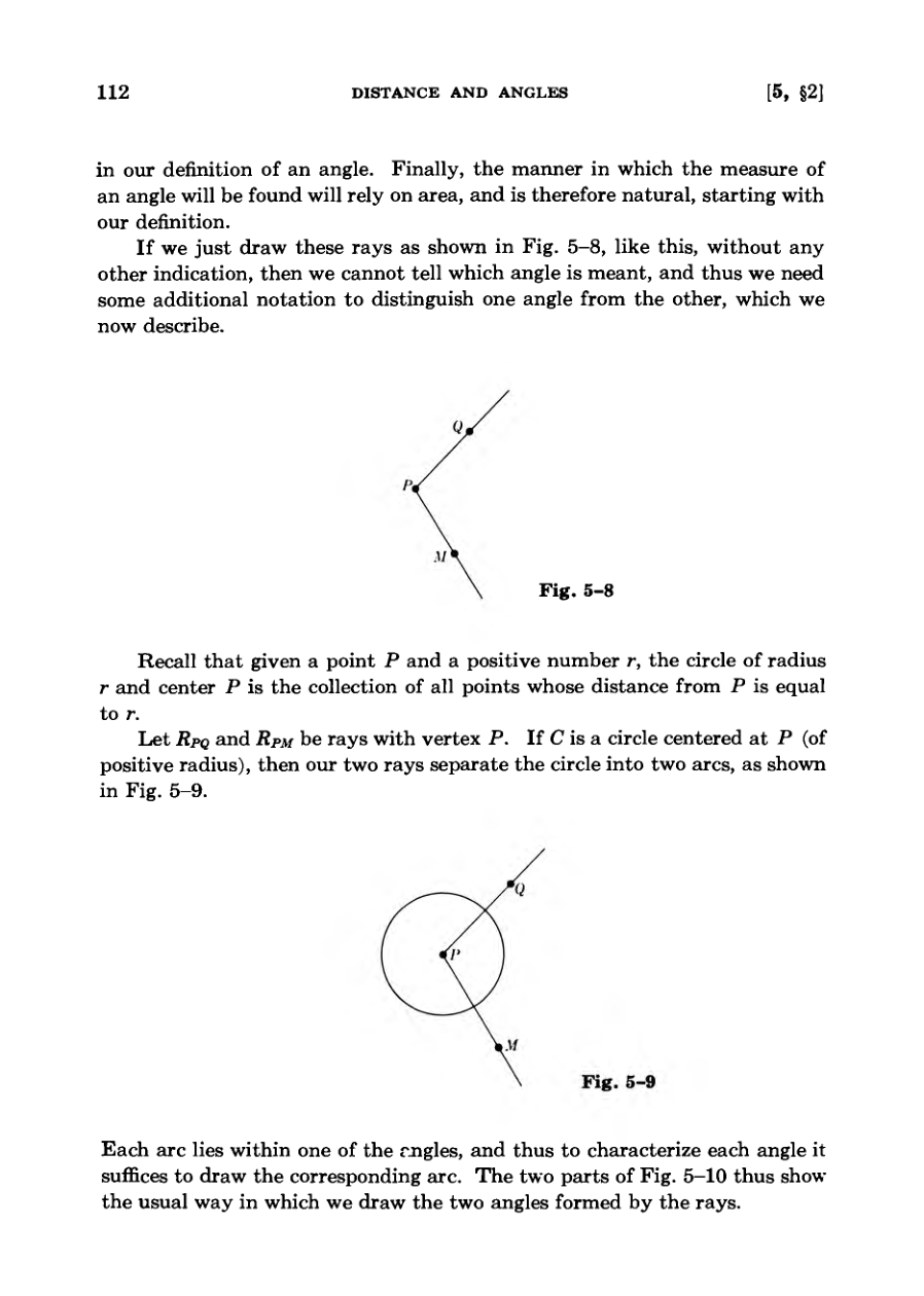
Incorporating additional information into the definition of an angle is necessary because rays alone do not indicate which specific angle is meant.
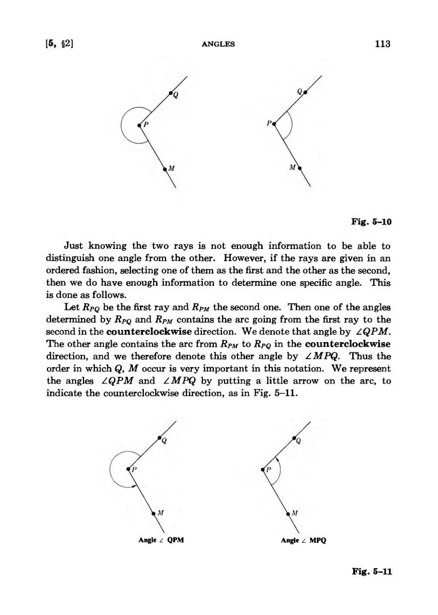
Using a circle centered at the vertex, rays separate the circle into two arcs, allowing each angle to be characterized by its corresponding arc.
Ordering the rays determines a specific angle by following the counterclockwise direction from the first ray to the second.
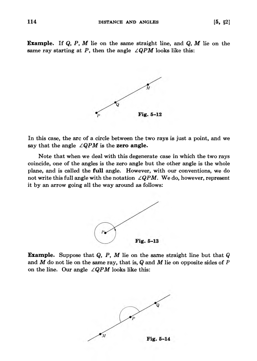
Degenerate cases like zero angles and full angles occur when the rays coincide along the same straight line.
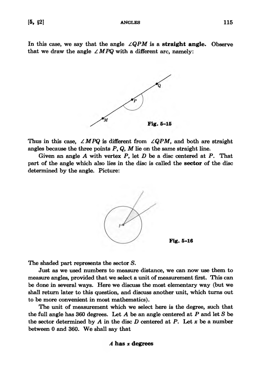
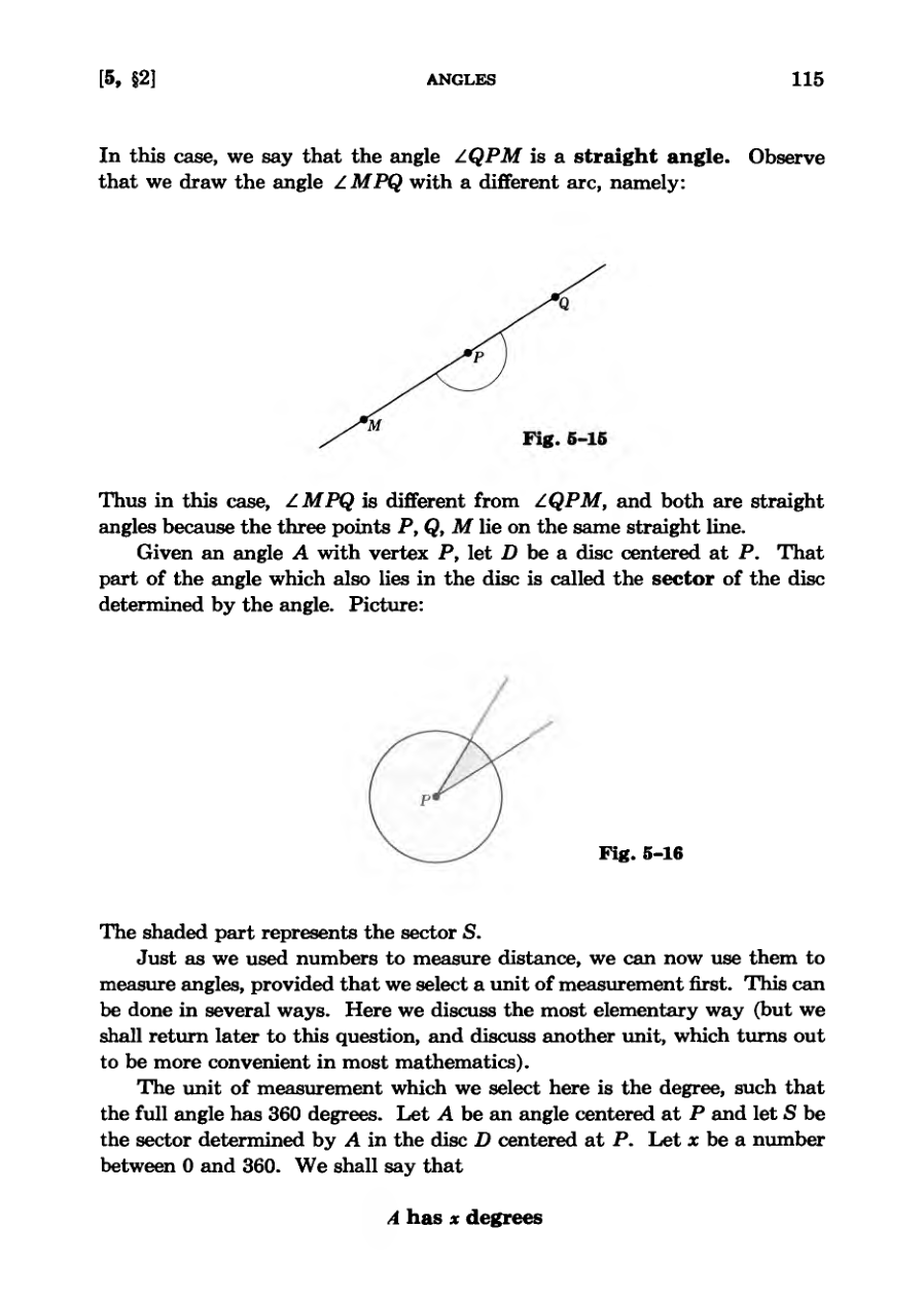
Straight angles arise when the points defining the rays lie on the same straight line but on opposite sides of the vertex.
A sector of a disc is defined as the portion of the angle that lies within a disc centered at the vertex.
Just knowing the two rays is not enough information to be able to distinguish one angle from the other.
DiagramDiagramDiagramDiagramDiagram
Measuring Angles with Degrees
Angles are measured using degrees, where a full angle consists of 360 degrees.
The degree measure of an angle is defined through the ratio of the area of its sector to the total area of the disc.
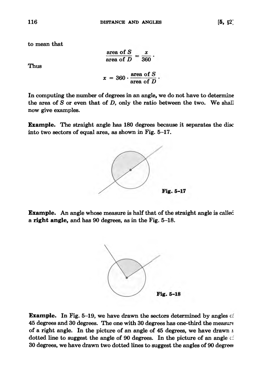
Special angles like straight angles and right angles correspond to 180 and 90 degrees respectively.
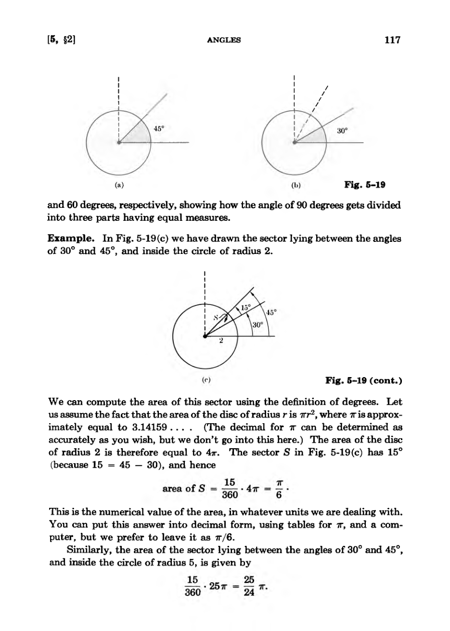
The area of a specific sector can be computed directly using its degree measure and the formula for the area of a disc.
Inequalities can be established between angles by comparing their numerical degree values.
In computing the number of degrees in an angle, we do not have to determine the area of S or even that of D, only the ratio between the two.
DiagramDiagramDiagram
Geometry Exercises and Triangles
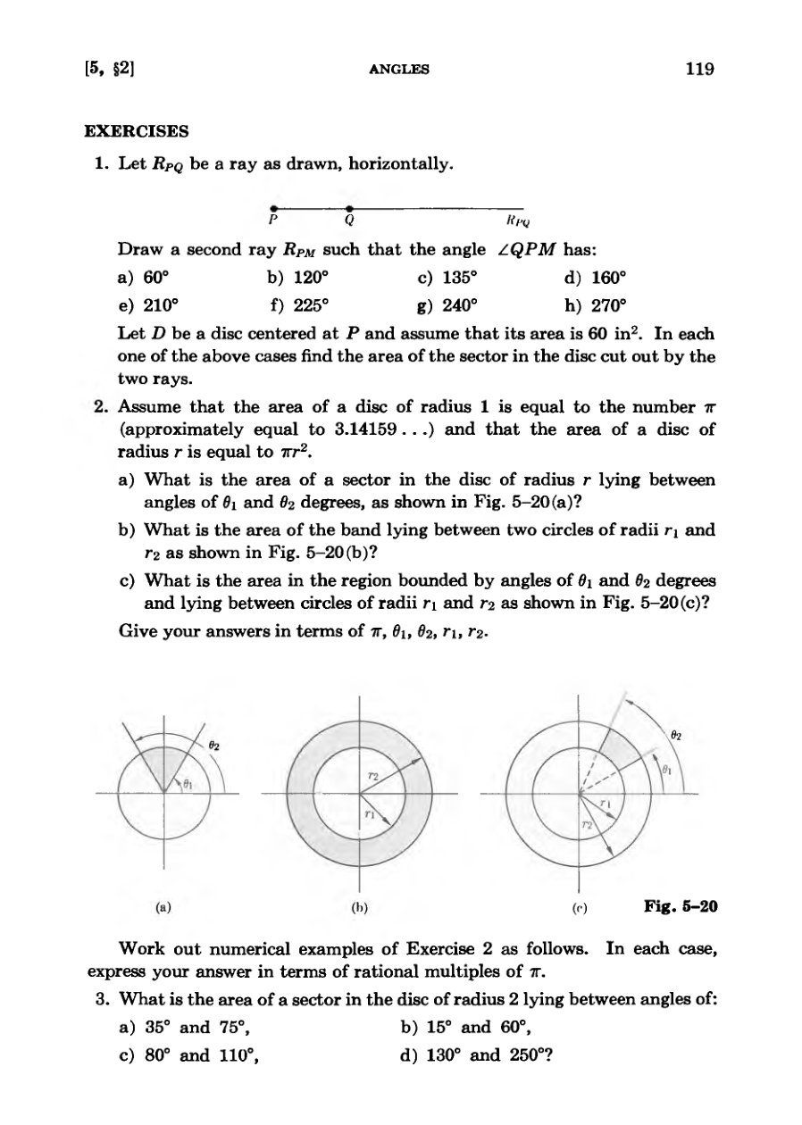
Students are asked to calculate the area of various disc sectors defined by specific angles.
Problems extend to finding the areas of circular bands and regions bounded by both angles and radii.
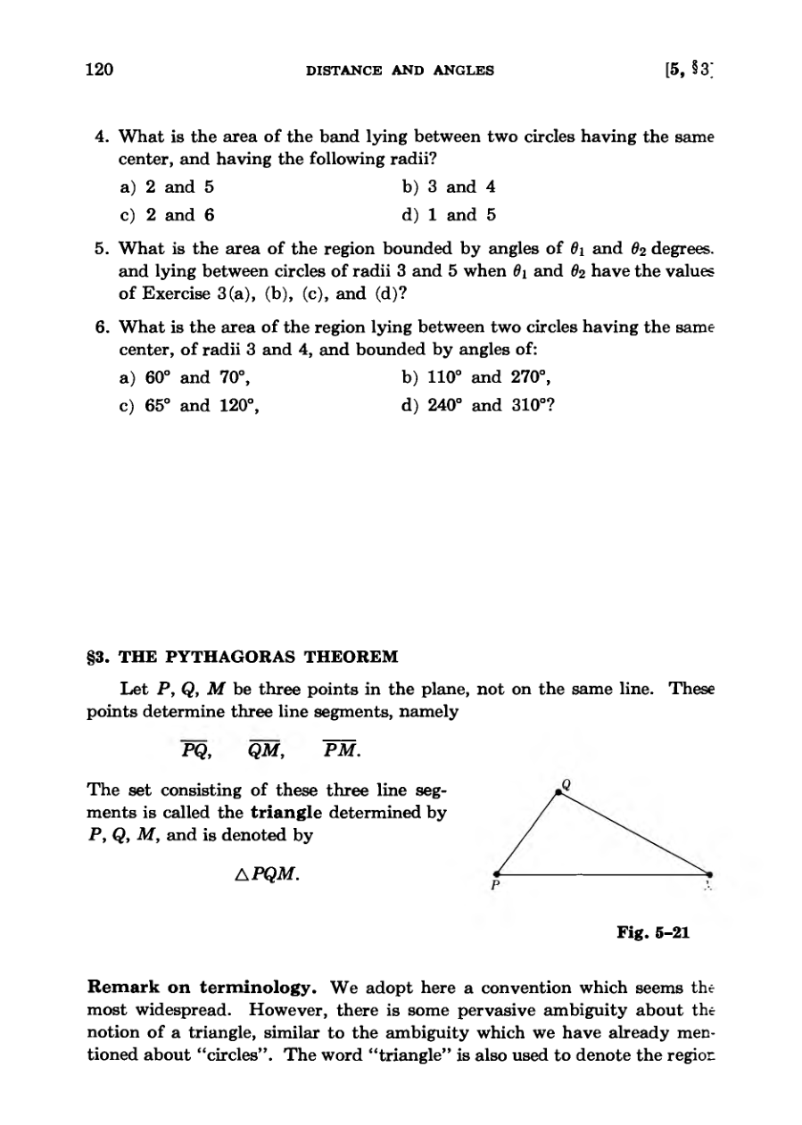
The text introduces the definition of a triangle formed by three non-collinear points.
The author discusses terminological ambiguity surrounding whether a triangle refers to its boundary or the enclosed region.
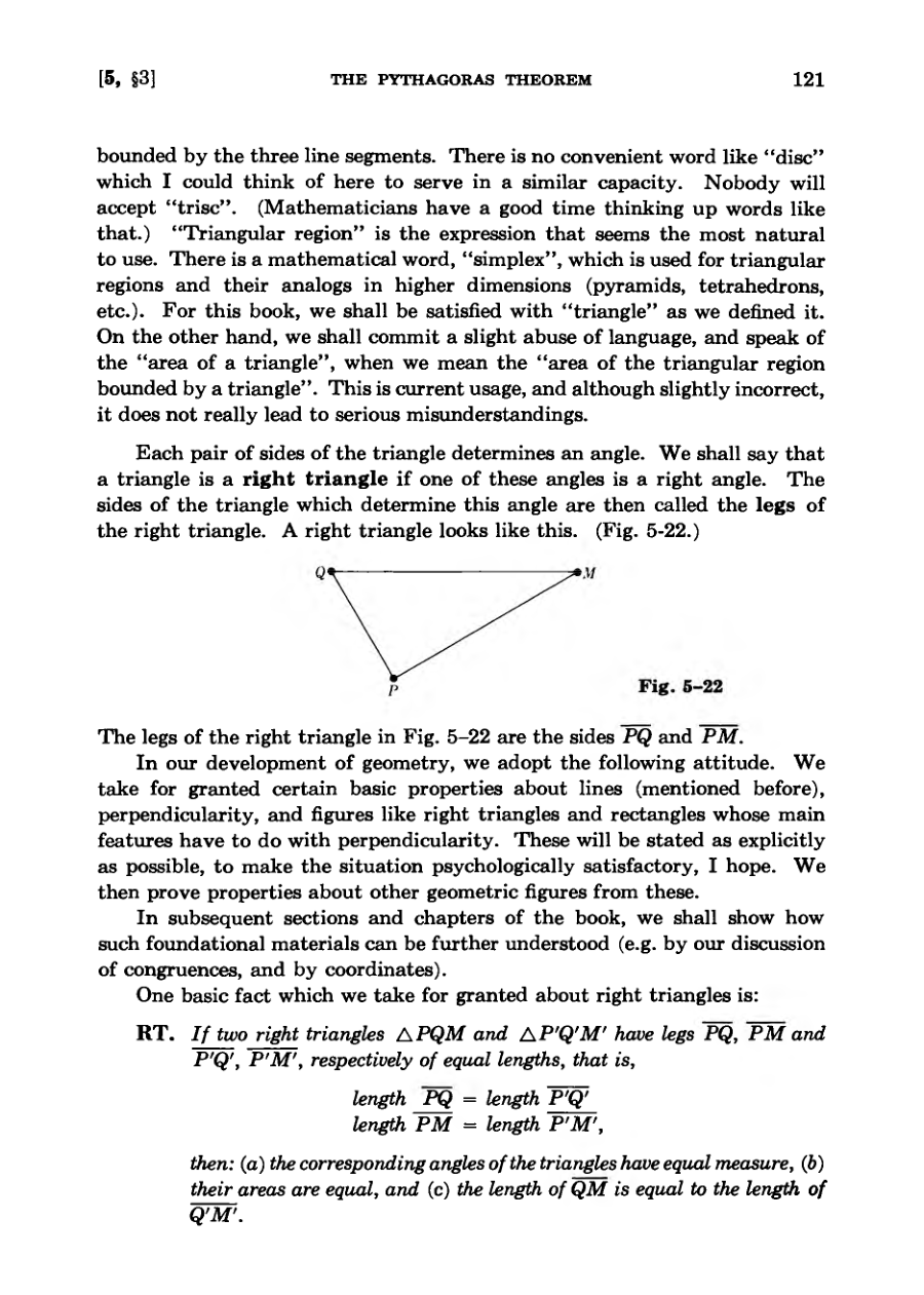
Right triangles and their legs are formally defined in preparation for exploring the Pythagorean theorem.
Nobody will accept 'trisc'.
DiagramFigureDiagram
Axioms of Geometry and Pythagoras
The text introduces foundational geometric principles, specifically focusing on right triangles through axiom RT.
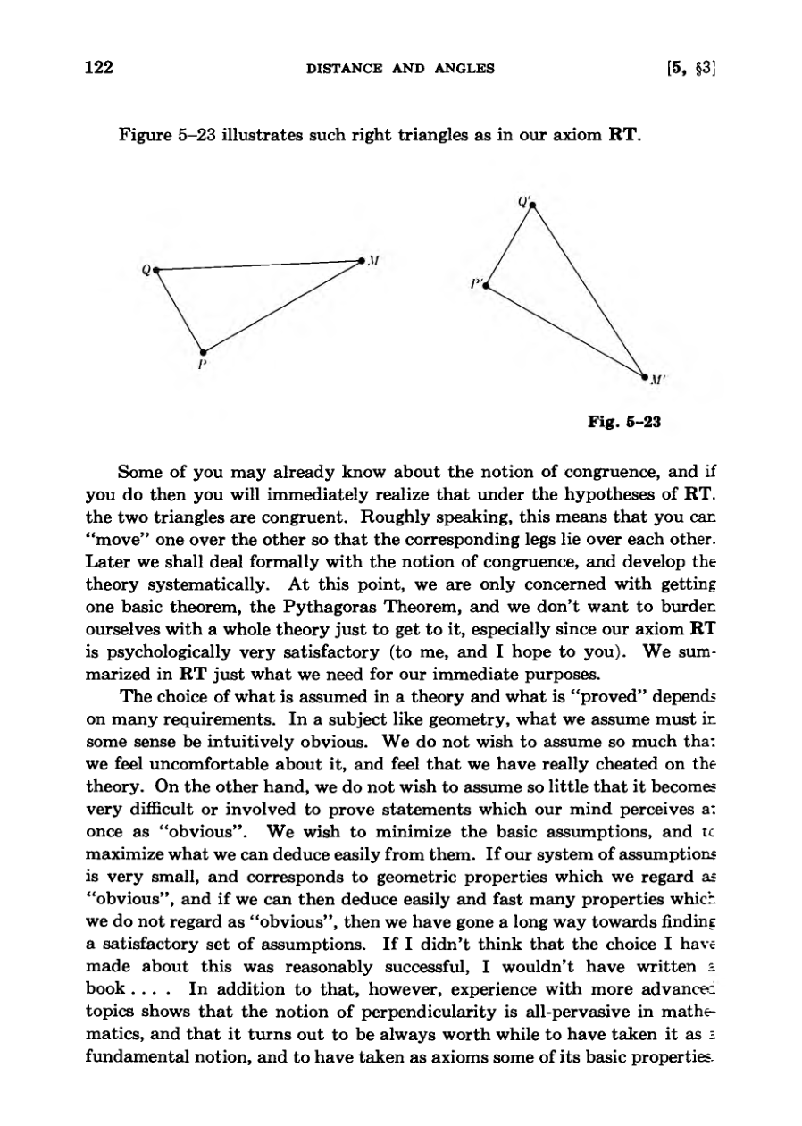
Axiom RT establishes that right triangles with equal legs share corresponding angle measures, areas, and hypotenuse lengths.
The author postpones a full formal theory of congruence to reach the Pythagorean theorem more directly.
Geometric theory balances minimizing basic assumptions with maximizing easily deduced properties that feel intuitively obvious.
Perpendicularity is highlighted as an all-pervasive and fundamental notion in advanced mathematics.
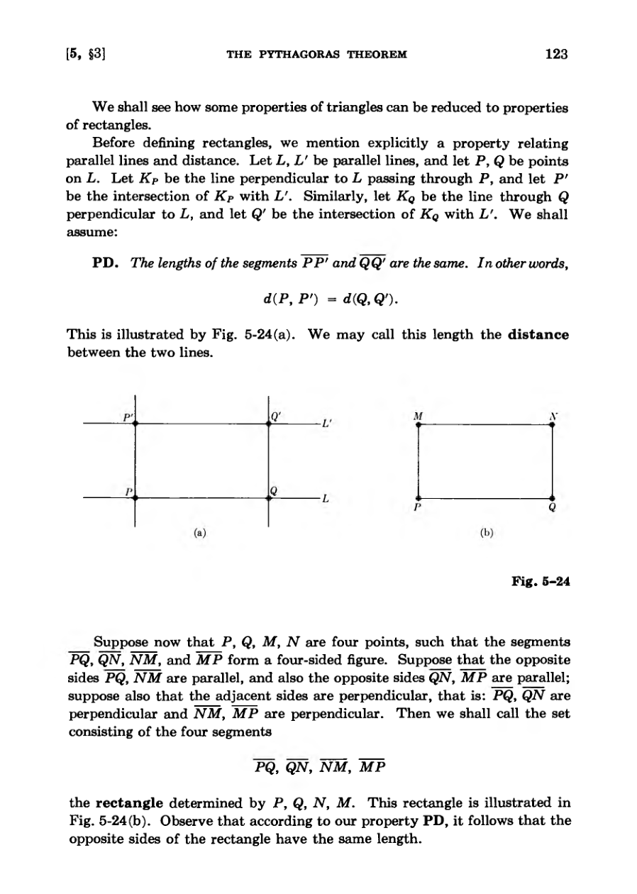
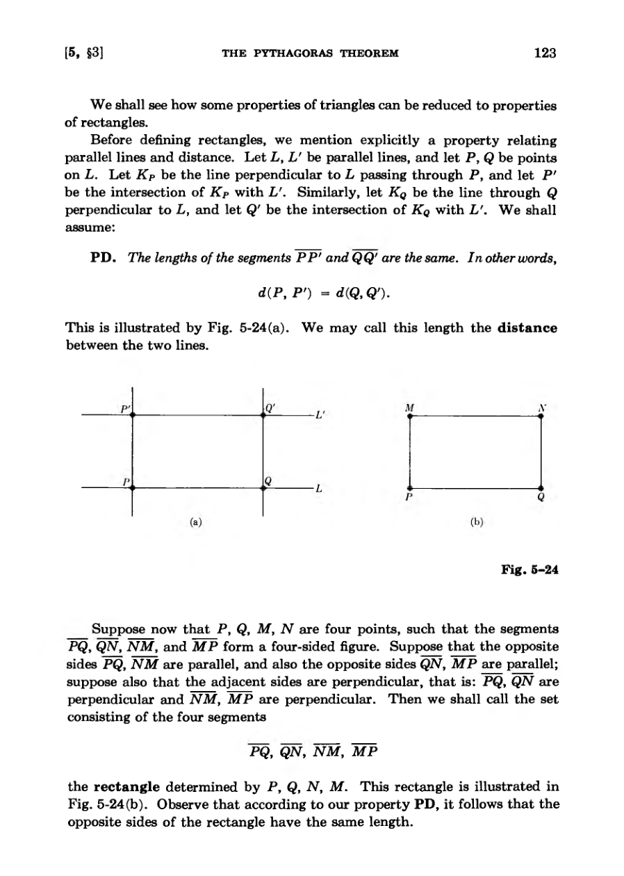
Additional assumptions, such as axiom PD, define properties of parallel lines and constant distance between them.
If I didn’t think that the choice I have made about this was reasonably successful, I wouldn’t have written a book . book . . .
DiagramDiagramDiagram
Geometry of Rectangles and Triangles
Defined the area of a rectangle as the product of its side lengths, ab.
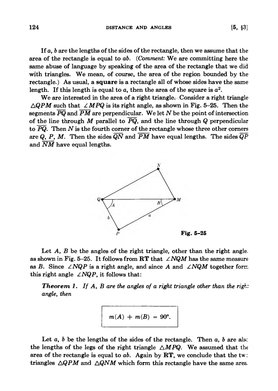
Established that the sum of the non-right angles in a right triangle equals ninety degrees.
Determined that the area of a right triangle with legs of lengths a and b is equal to one-half of ab.
Introduced the Pythagorean theorem, relating the lengths of the legs and the hypotenuse of a right triangle.
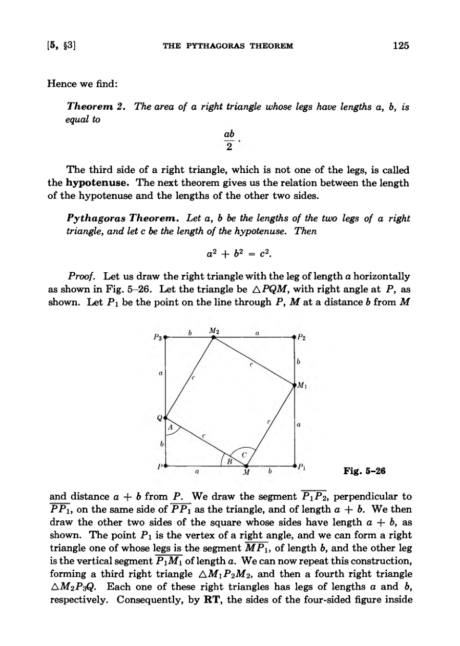
Outlined the geometric construction used to prove that a squared plus b squared equals c squared.
We are committing here the same abuse of language by speaking of the area of the rectangle that we did with triangles.
DiagramDiagramDiagram
The Pythagorean Theorem
The text demonstrates the geometric proof of the Pythagorean theorem relating the sides of a right triangle.
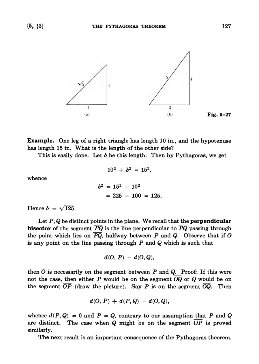
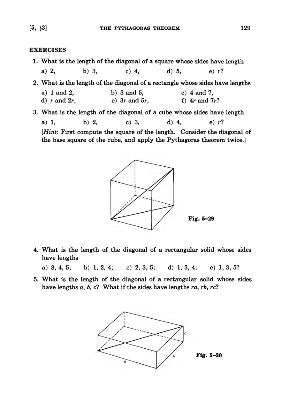
Practical applications include calculating the lengths of diagonals for squares, rectangles, and right triangles.
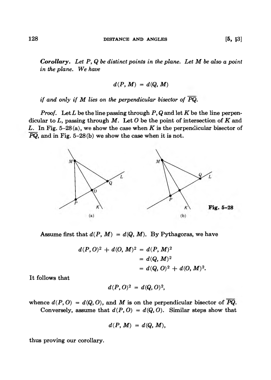
Properties of the perpendicular bisector of a line segment are defined and proven using distance equations.
A corollary establishes that a point is equidistant from two points if and only if it lies on their perpendicular bisector.
Comprehensive exercises apply these geometric principles to various figures, solids, and real-world distance problems.
Observe that if O is any point on the line passing through P and Q which is such that d(O,P) = d(O,Q), then O is necessarily on the segment between P and Q.
DiagramDiagramDiagramDiagram
Geometry Exercises and Isometries
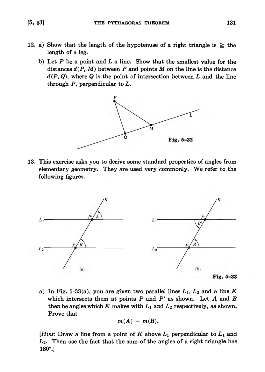
Practices applying the Pythagorean theorem to calculate kite string lengths and heights.
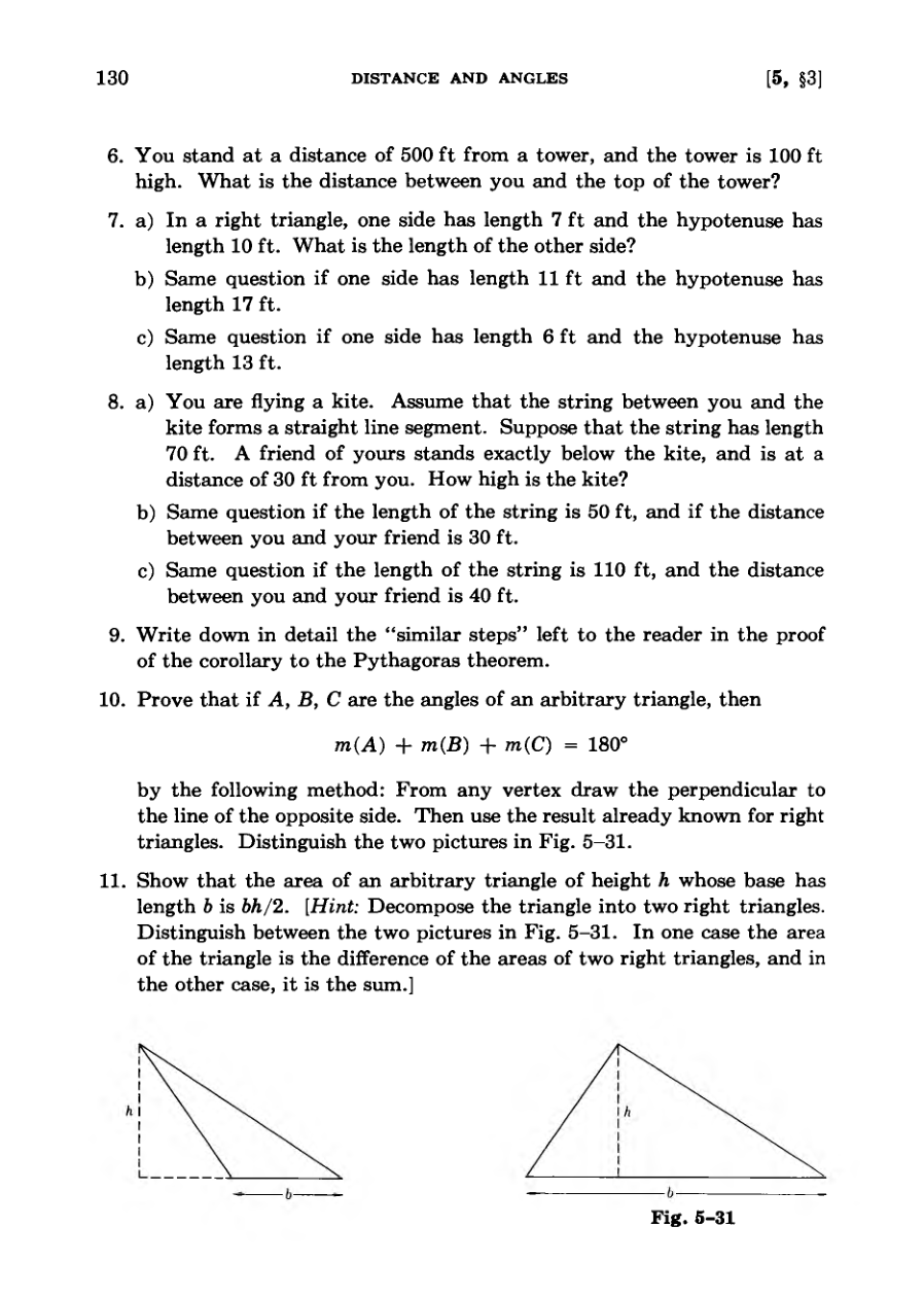
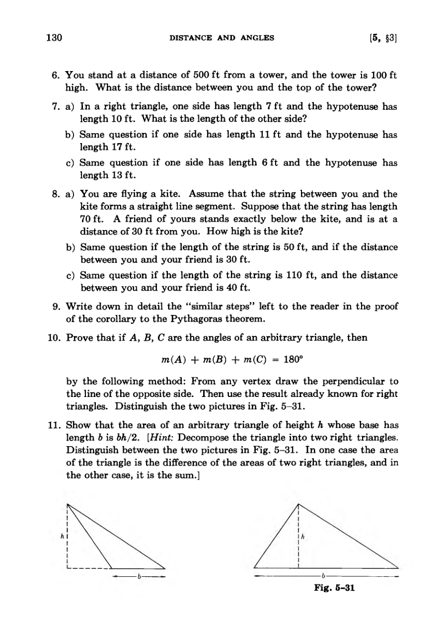
Proves foundational geometric properties including the sum of angles in a triangle and triangle area formulas.
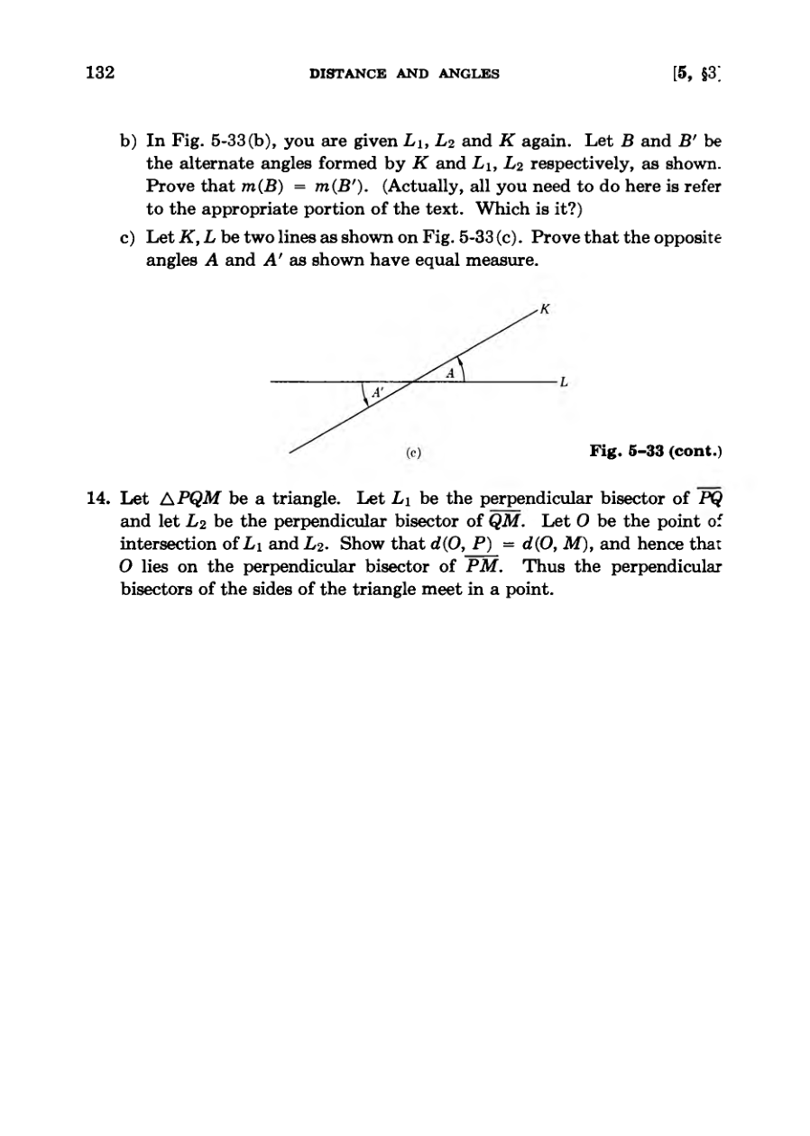
Derives standard properties of angles formed by parallel lines and transversals.
Explores the intersection of perpendicular bisectors in triangles.
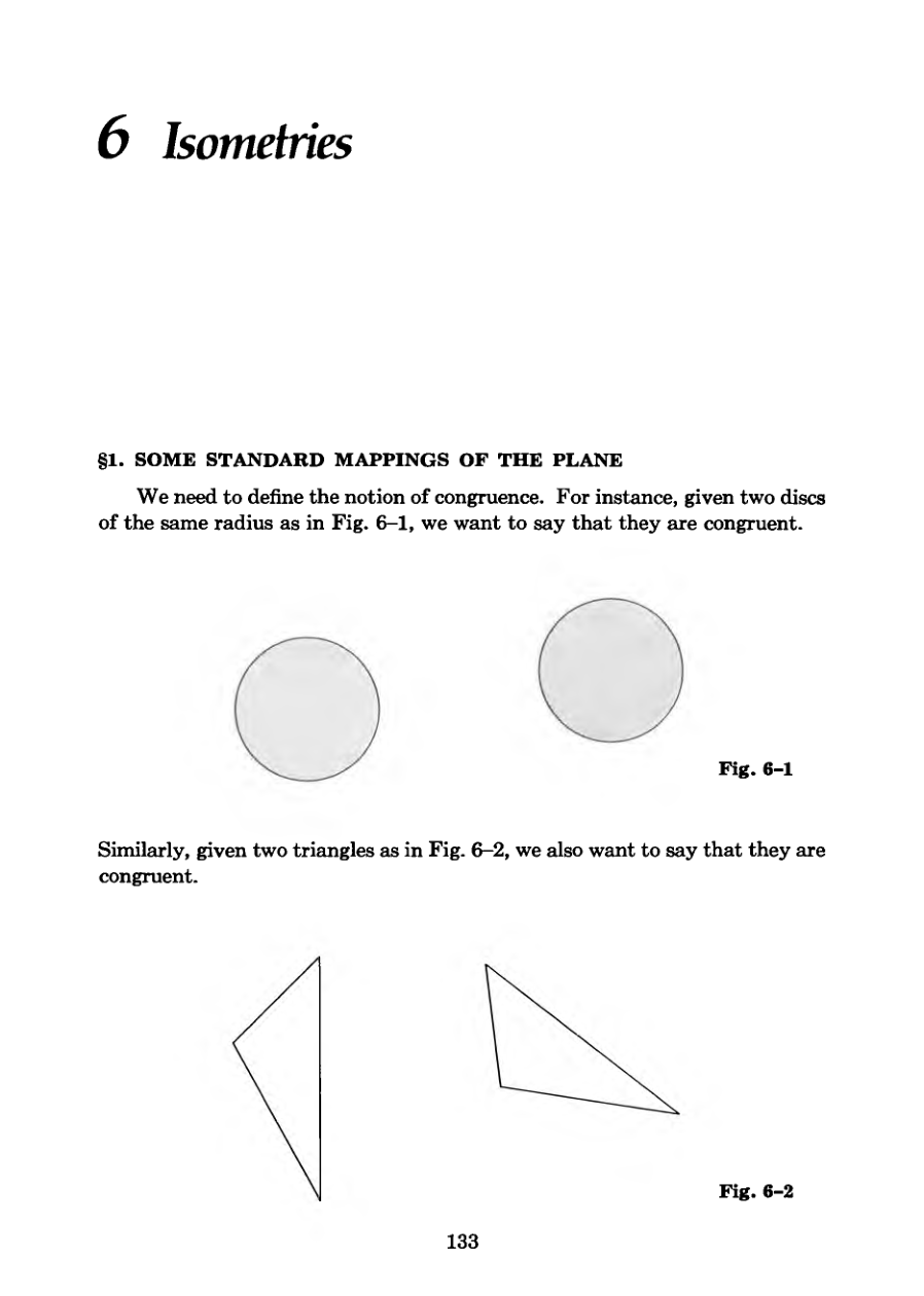
Introduces the concept of congruence through visual examples like discs and triangles.
Defines the foundational concepts of mappings, isometries, and transformations in the plane.
Roughly speaking, this means that one figure can be laid over the other.
DiagramDiagramDiagramDiagram
Standard Mappings in Geometry
Mappings associate each point in the plane with a corresponding value or image point.
Constant mappings assign every point in the plane to a single fixed point O.
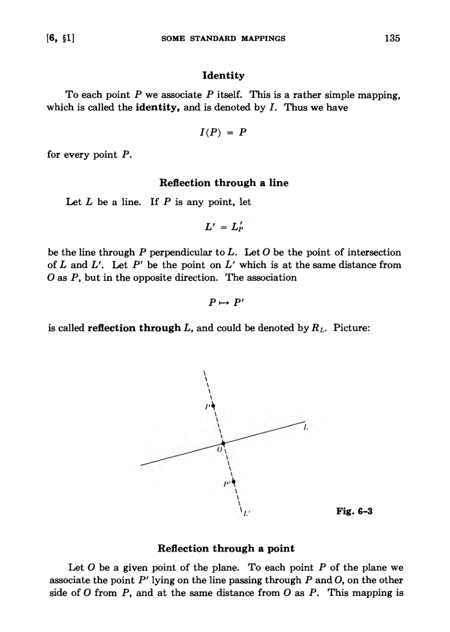
The identity mapping simply associates every point P with itself.
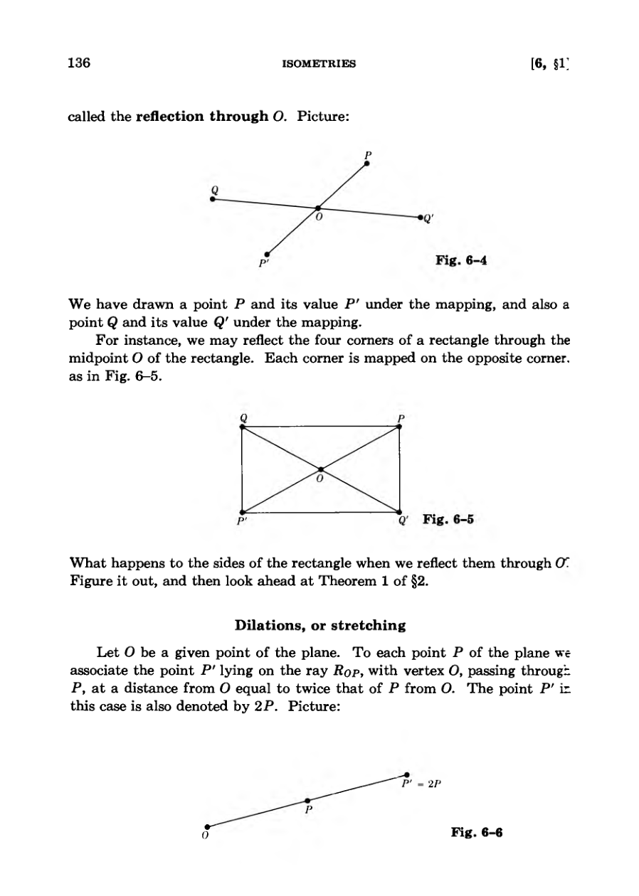
Reflections map points across either a given line or a fixed central point.
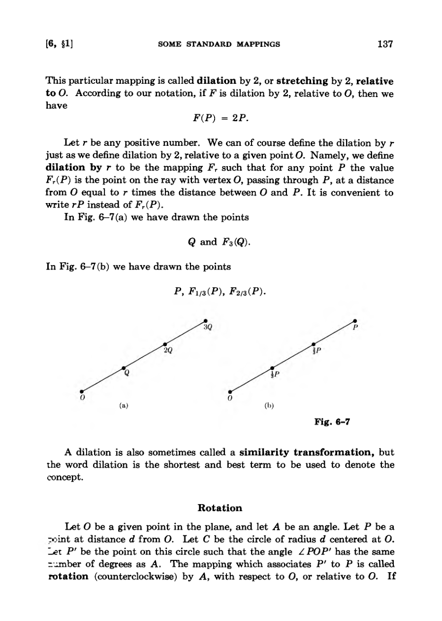
Dilations stretch or shrink distances from a fixed point by a positive scale factor r.
Rotations move points along a circle around a center point by a specified angle.
A dilation is also sometimes called a similarity transformation, but the word dilation is the shortest and best term to be used to denote the concept.
DiagramDiagramDiagram
Defining Geometric Rotations
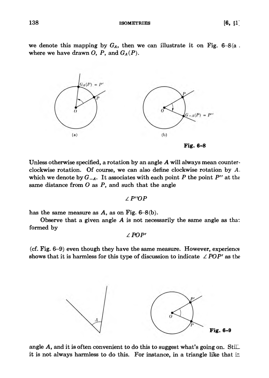
Rotations are formally defined as mappings that move points around a center by specific angles in counterclockwise or clockwise directions.
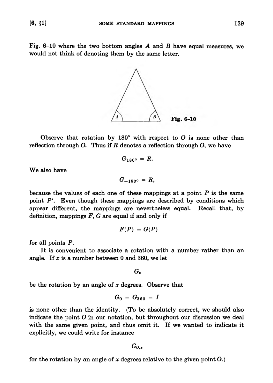
Equal measures do not automatically mean two angles are identical objects, requiring care in notation and context.
A 180-degree rotation around a center point is mathematically equivalent to a reflection through that same point.
Rotations can be conveniently associated with numerical values of degrees rather than geometric angles.
Arbitrary or negative numbers of degrees are normalized using multiples of 360 to determine the equivalent standard rotation.
Observe that rotation by 180° with respect to O is none other than reflection through O.
DiagramDiagramDiagram
Understanding Plane Isometries
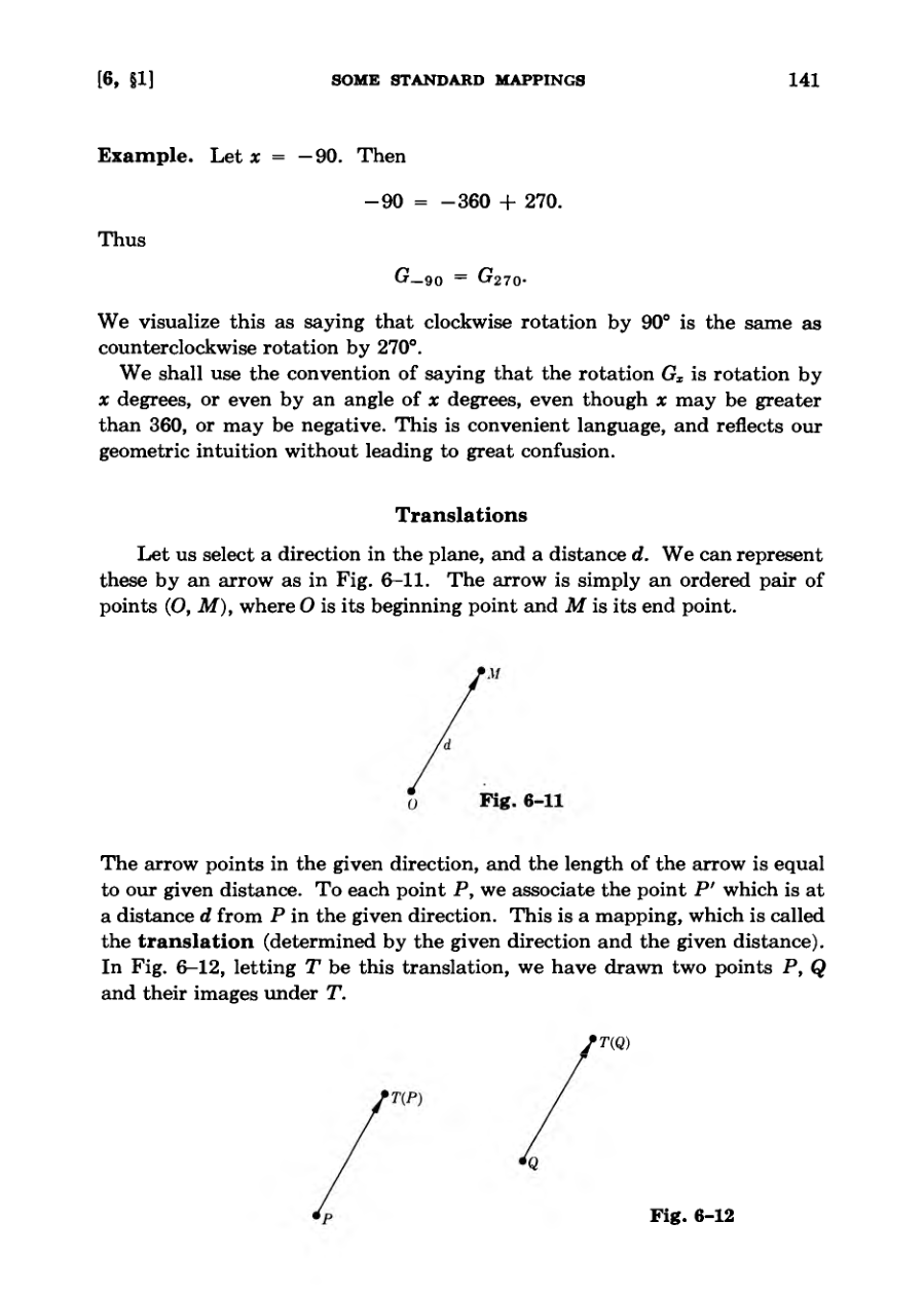
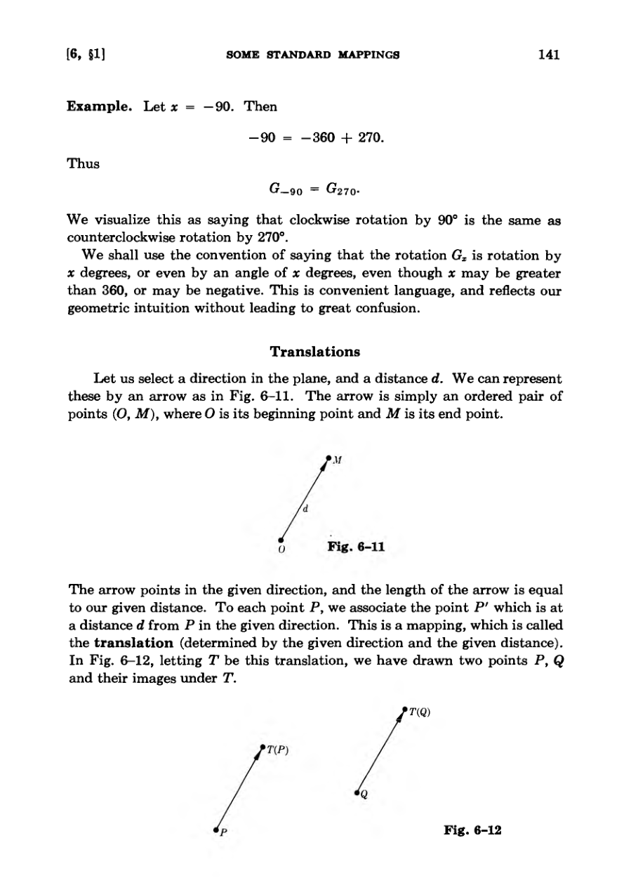
A translation in the plane associates each point with another by a specific direction and distance represented by an arrow.
Mappings like translations, reflections, and rotations have unique fixed point characteristics depending on their geometric definition.
An isometry is defined as a mapping of the plane into itself that strictly preserves the distances between every pair of points.
Common transformations such as point reflections, line reflections, rotations, and translations all qualify as isometries.
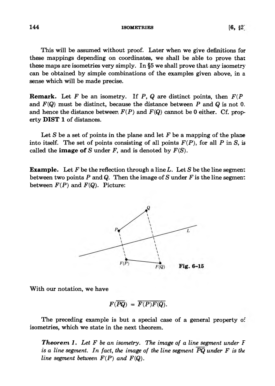
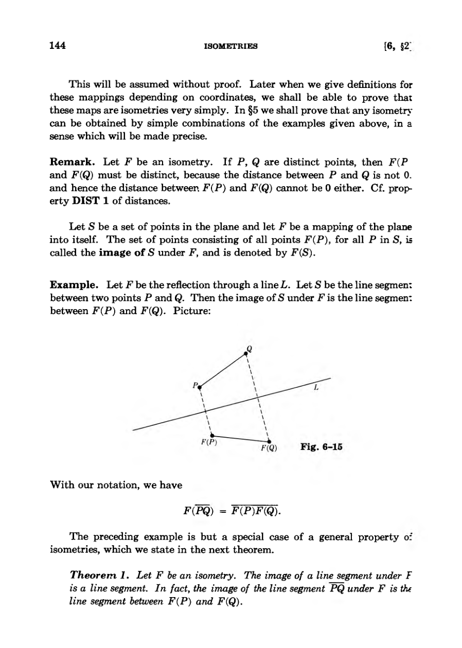
Mapping images of sets, such as line segments under reflections, preserve geometric integrity through distance preservation.
Let F be a mapping of the plane into itself. We say that F preserves distances, or is distance preserving, if and only if for every pair of points P, Q in the plane, the distance between P and Q is the same as the distance between F(P) and F(Q).
DiagramFigureDiagramFigure
Properties of Isometries
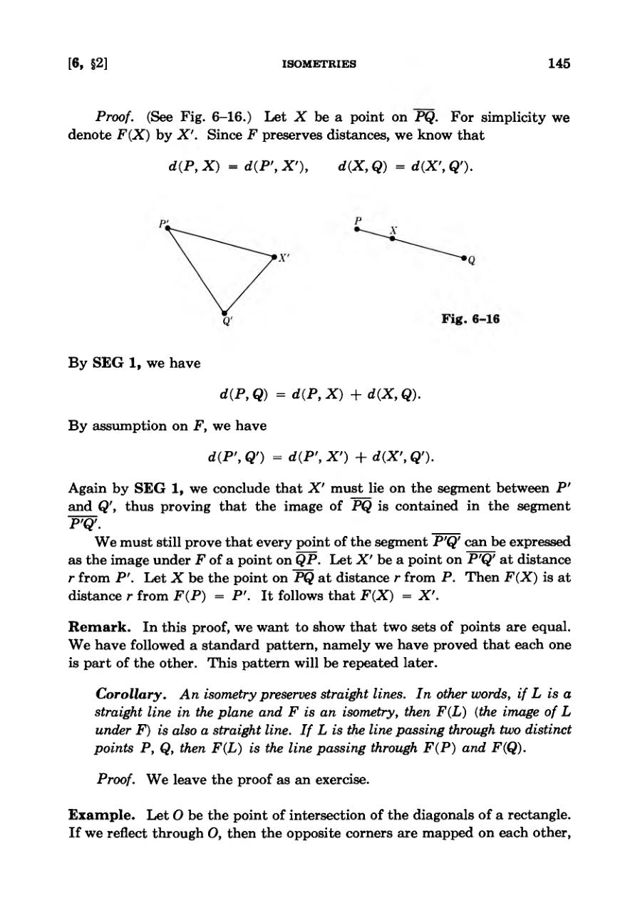
Theorem 1 establishes that the image of a line segment under an isometry is also a line segment between the respective image endpoints.
Proving set equality in the theorem follows a standard mathematical pattern by showing each set is contained within the other.
A corollary to the theorem proves that isometries preserve straight lines in the plane.
Fixed points of isometries play a crucial role in systematically describing and analyzing all types of isometries.
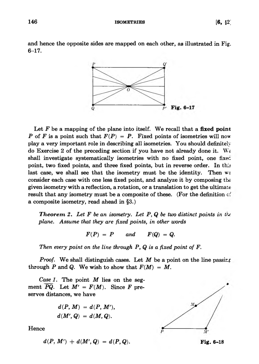
Theorem 2 demonstrates that if two distinct points are fixed by an isometry, every point on the line passing through them is also a fixed point.
In this proof, we want to show that two sets of points are equal.
FigureDiagramDiagramDiagram
Theorem 3 and Composition of Isometries
Theorem 3 establishes that an isometry is the identity mapping if it fixes three distinct non-collinear points.
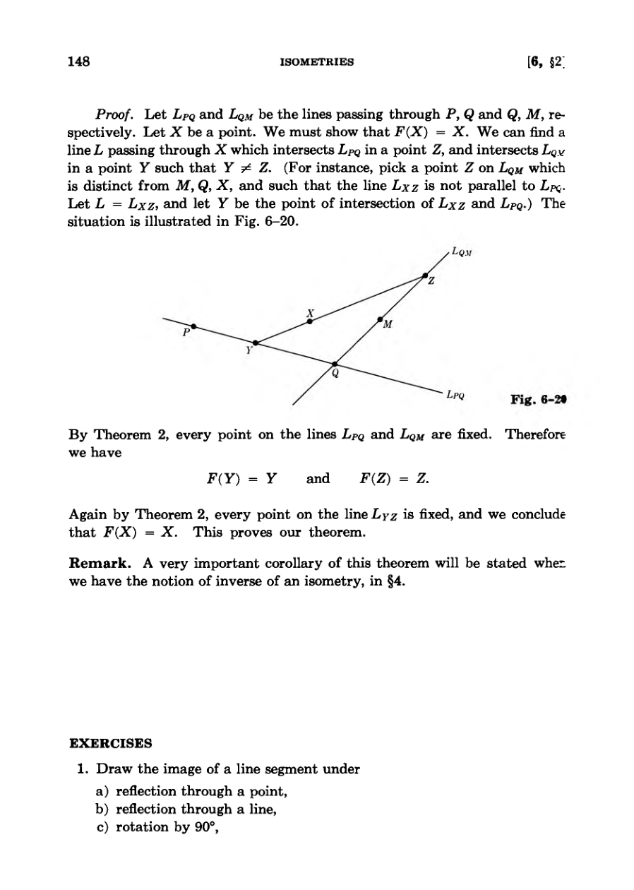
The proof constructs intersecting lines through fixed points to demonstrate that any arbitrary point must also be fixed.
Exercises at the end of the section challenge readers to apply transformations to lines, circles, and parallel structures.
An extension exercise invites generalization of these planar isometry theorems into three-dimensional space.
Section 3 introduces the composition of isometries, describing how applying transformations in succession yields a new mapping.
We can find a line L passing through X which intersects LPQ in a point Z, and intersects LQM in a point Y such that Y != Z.
DiagramDiagramDiagram
Composition of Isometries
The composite of two isometries F and G, denoted F o G, represents applying G first and then F.
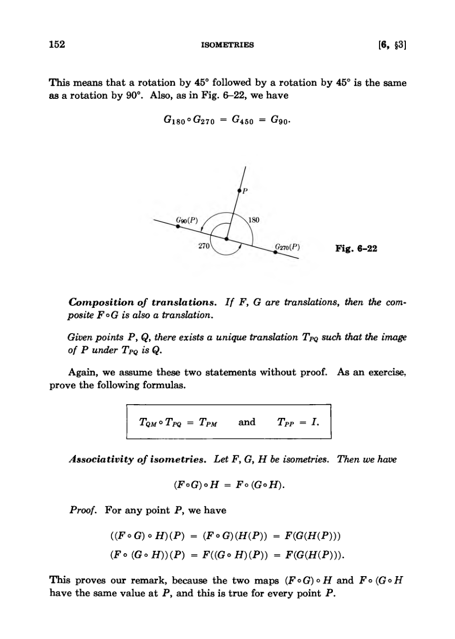
Composing rotations or translations around the same center results in another rotation or translation.
The composition of rotations behaves analogously to the addition of angles.
The composition of isometries is associative, allowing consistent grouping without changing the result.
Iterating an isometry multiple times creates powers that mirror algebraic exponent rules like F^(m+n) = F^m o F^n.
Note this interesting cyclical nature of F, that F5 = F.
DiagramDiagram
Geometry and Isometry Exercises
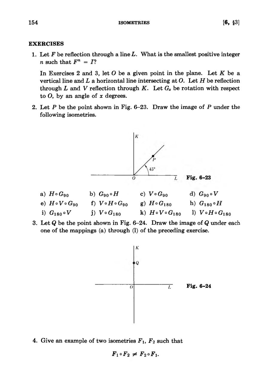
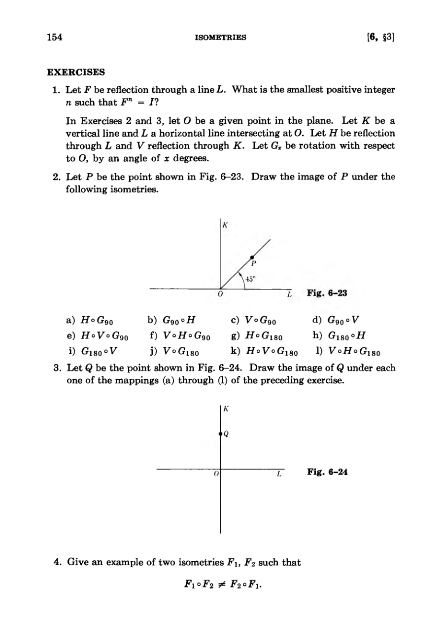
Exercises involve applying reflections, rotations, and their compositions to points in the plane.
Problems require finding specific image coordinates or patterns using geometric transformations like translations and rotations.
One exercise asks for an example demonstrating that the composition of two isometries is not always commutative.
An inverse function reverses the mapping of points, such that if P equals F of Q, then Q equals the inverse of F of P.
Reflections act as their own inverse because applying the reflection twice results in the identity transformation.
Rotations have inverses corresponding to rotations in the opposite direction by the same angle.
Draw a small flower. Let T be translation by 1 in. to the right, and let U be translation by 1 in. vertically upward.
DiagramDiagram
Inverse and Equality of Isometries
The concept of inverse translations is introduced, showing how operations like moving right have direct inverse operations moving left.
A corollary to Theorem 3 demonstrates that if two isometries map three non-collinear points to the same locations and an inverse exists, the isometries are identical.
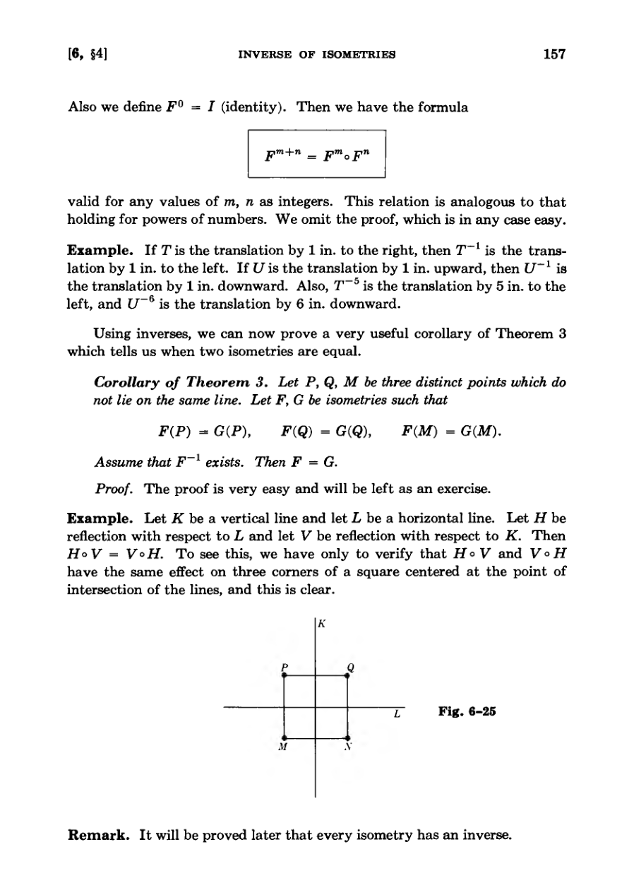
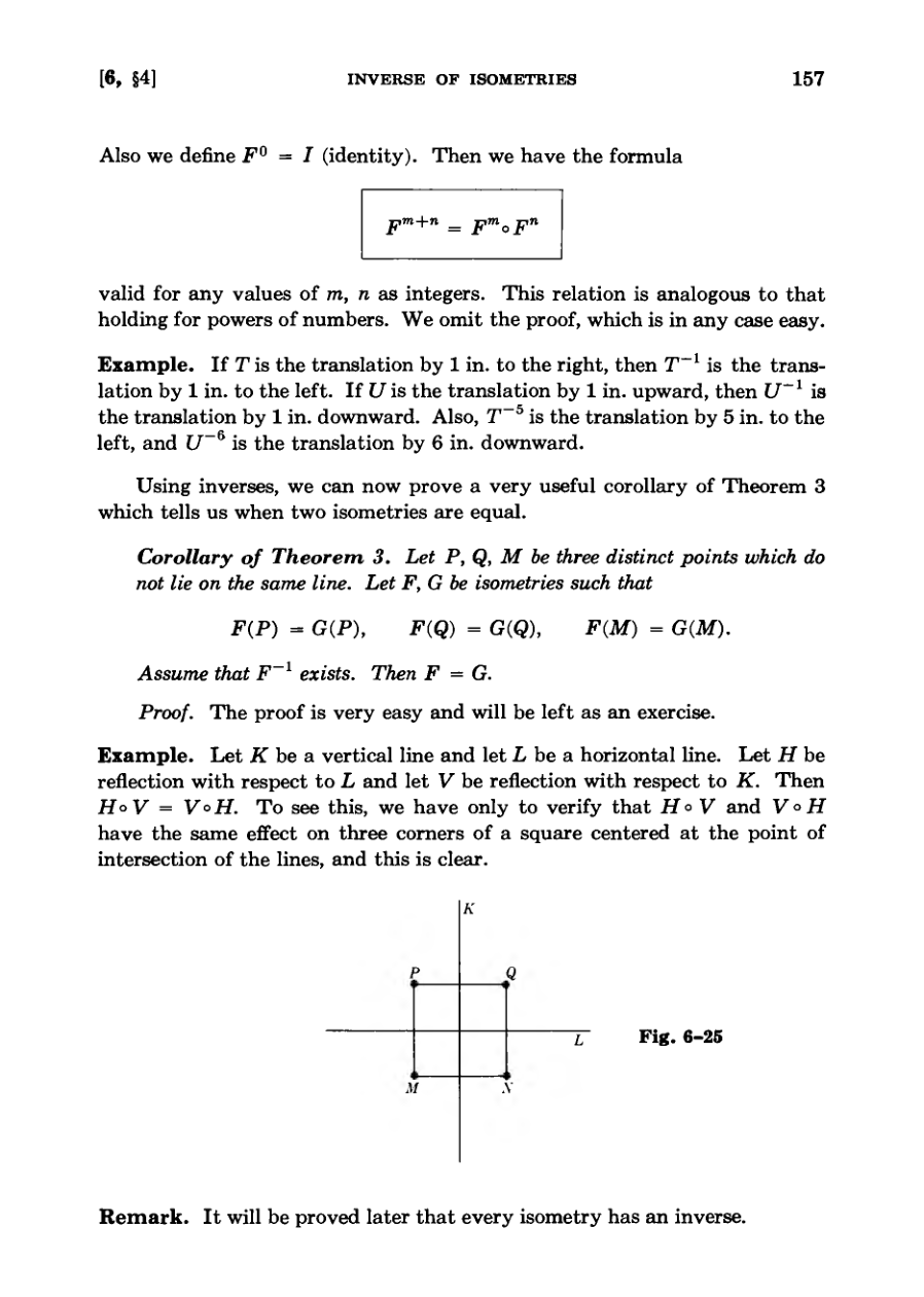
Examples involving horizontal and vertical reflections illustrate the commutative property under specific geometric configurations.
Exercises prompt the reader to prove properties of circles and discs under invertible isometries.
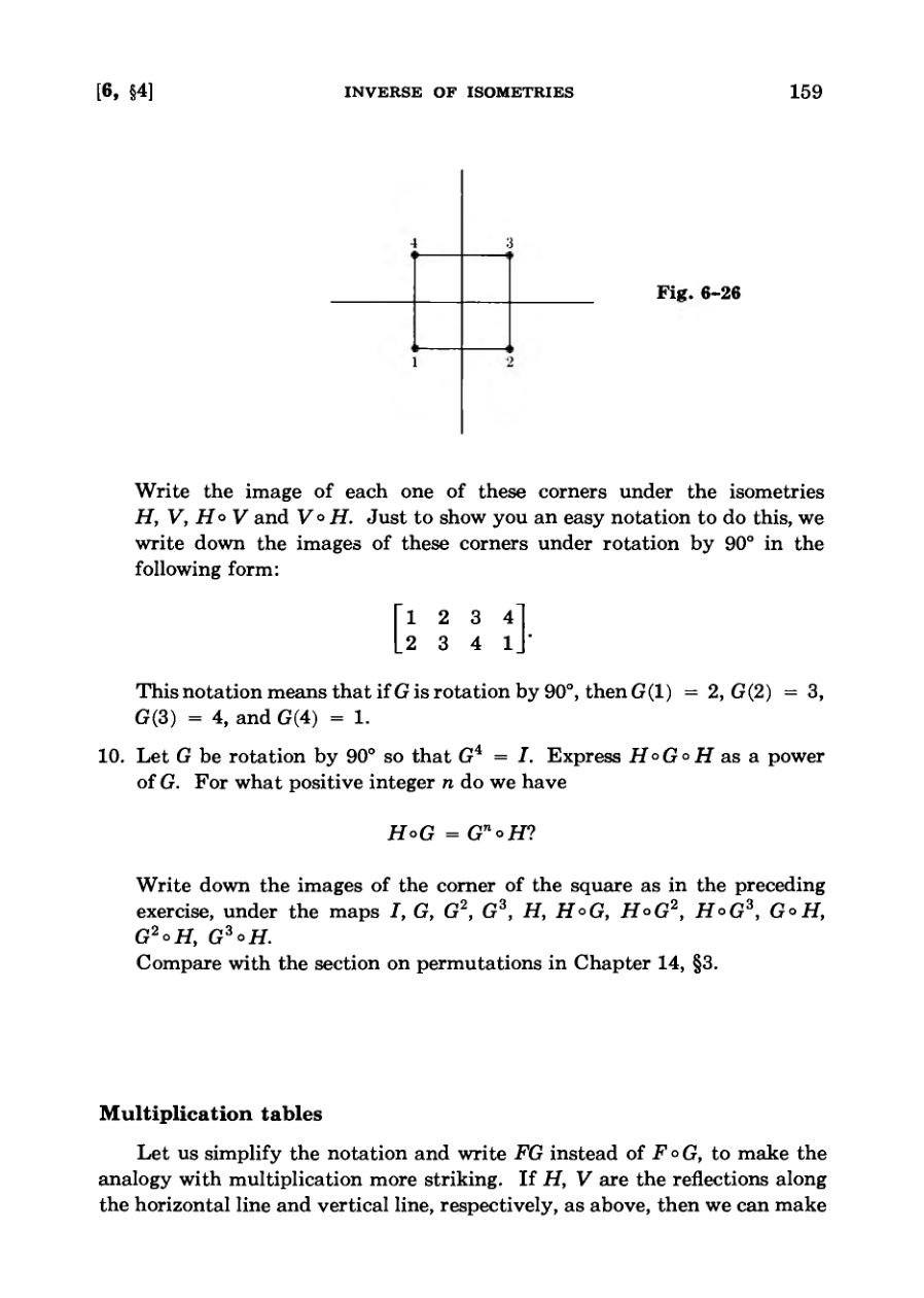
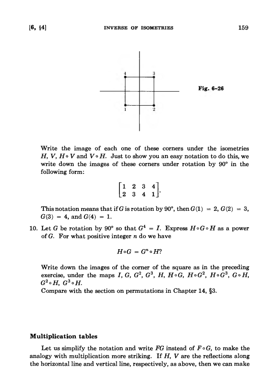
Further exercises explore cancellation laws, powers of isometries, and matrix-like permutation notations for geometric transformations.
Using inverses, we can now prove a very useful corollary of Theorem 3 which tells us when two isometries are equal.
DiagramDiagram
Multiplication Tables and Isometries
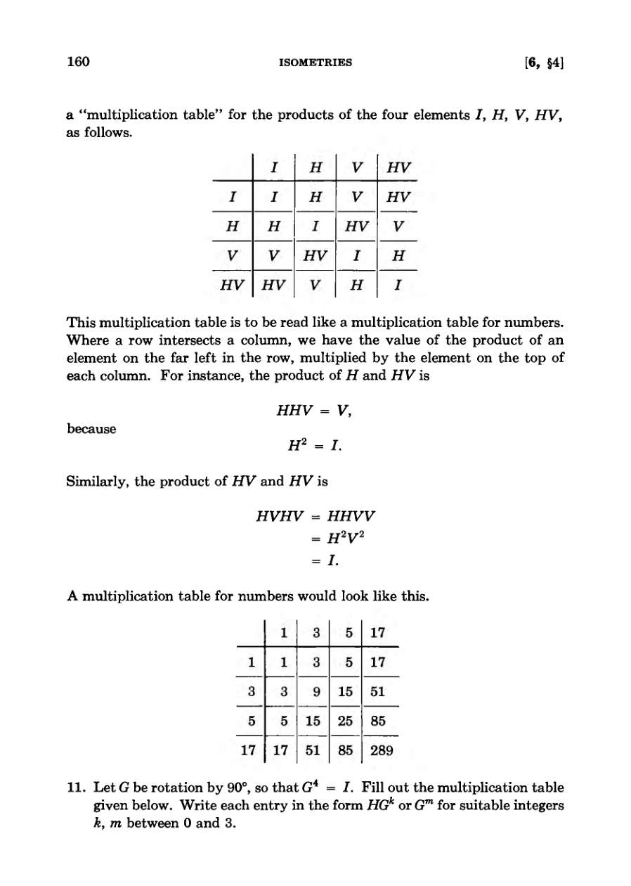
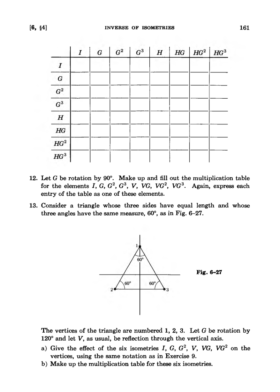
Constructing multiplication tables for combinations of horizontal and vertical line isometries.
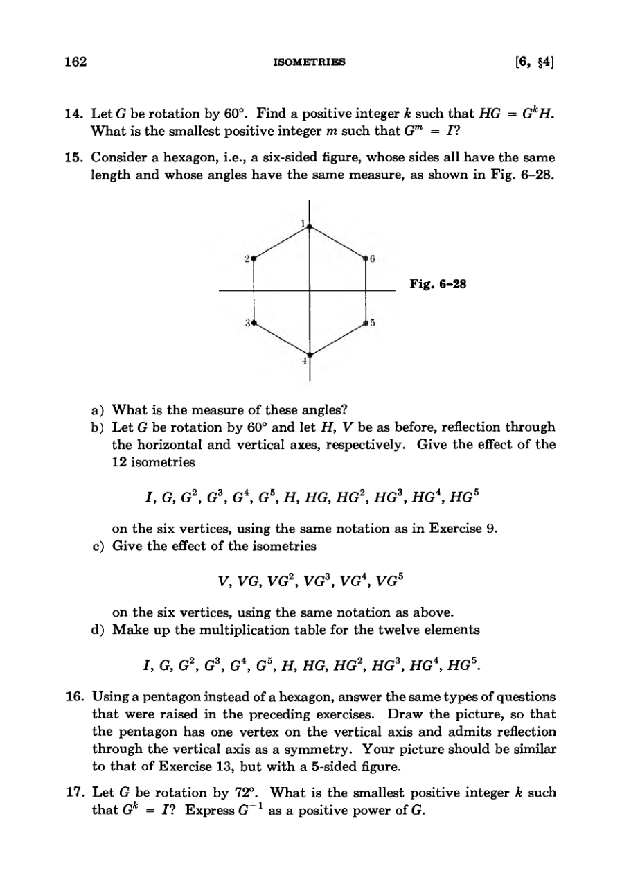
Applying rotation and reflection operations to geometric shapes like triangles, pentagons, and hexagons.
Solving exercises involving powers of rotations and explicit isometry compositions on vertices.
Introducing the characterization of isometries as composites of translations, rotations, and reflections.
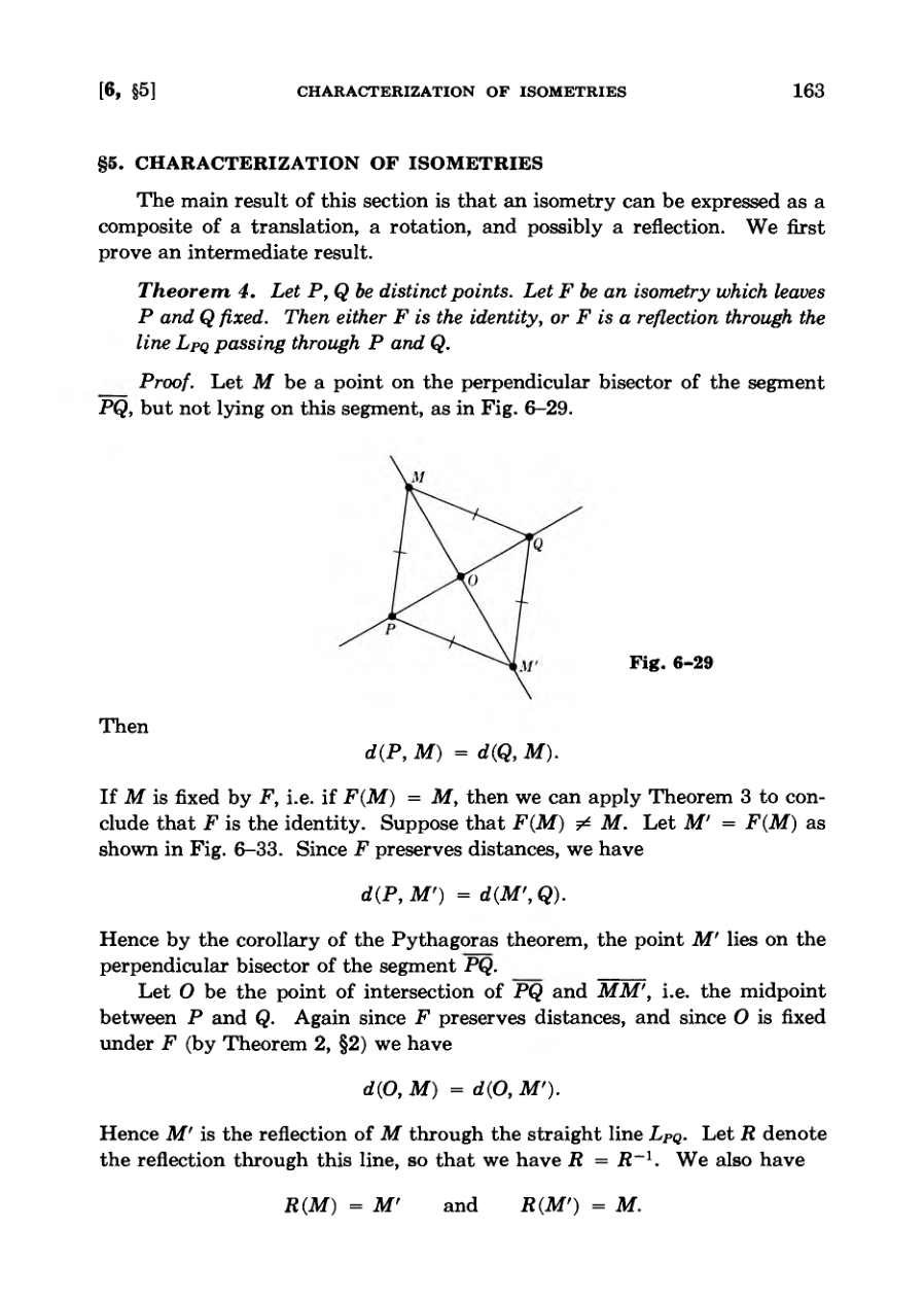
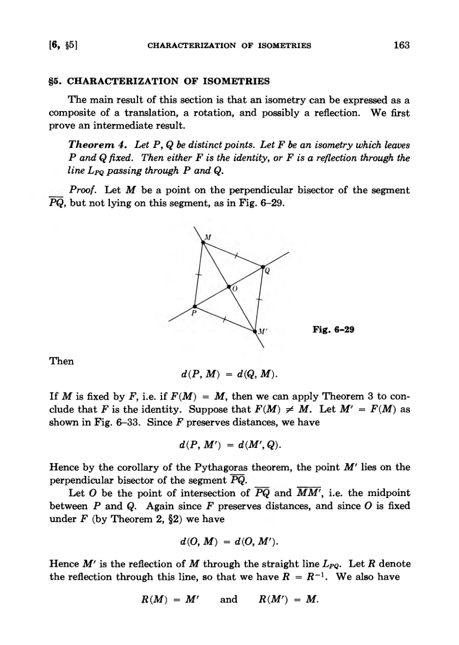
Proving Theorem 4 regarding isometries that leave two distinct points fixed.
The main result of this section is that an isometry can be expressed as a composite of a translation, a rotation, and possibly a reflection.
DiagramDiagramDiagramDiagramDiagram
Characterization and Congruence of Isometries
Theorem 4 establishes that an isometry leaving two points fixed is a reflection.
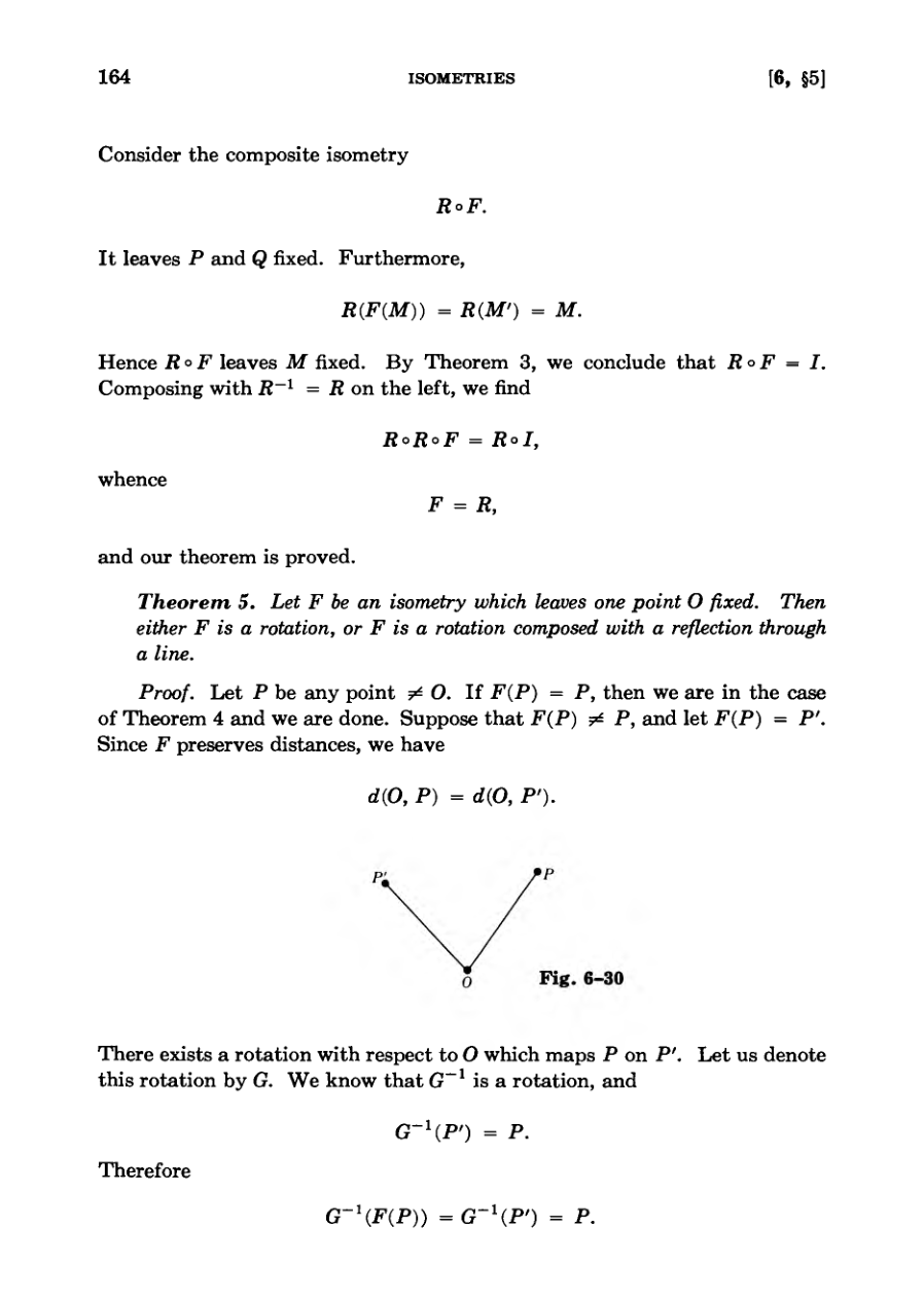
Theorem 5 proves that any isometry leaving one point fixed is either a rotation or a rotation composed with a reflection.
Theorem 6 classifies an arbitrary isometry without fixed points as a translation, a translation combined with a rotation, or further combined with a reflection.
Section 6 introduces congruences of point sets in the plane, defining them through the existence of an isometry.
Theorem 7 demonstrates that two circles of the same radius are congruent by using a distance-preserving translation.
If F does not leave any point fixed, then F is either a translation, or the composite of a translation and a rotation, or the composite of a translation, a rotation, and a reflection through a line.
DiagramDiagramFigure
Geometric Congruence Proofs
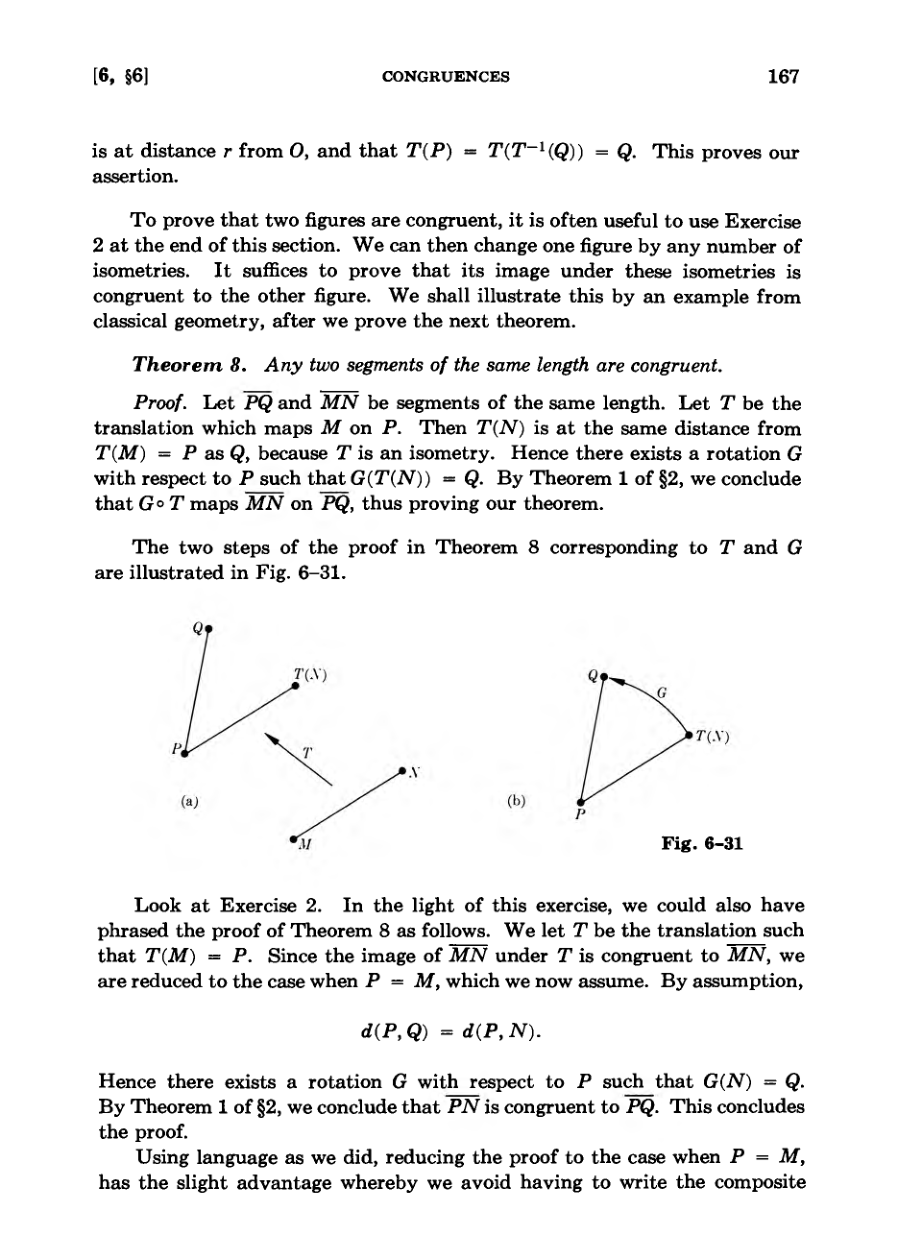
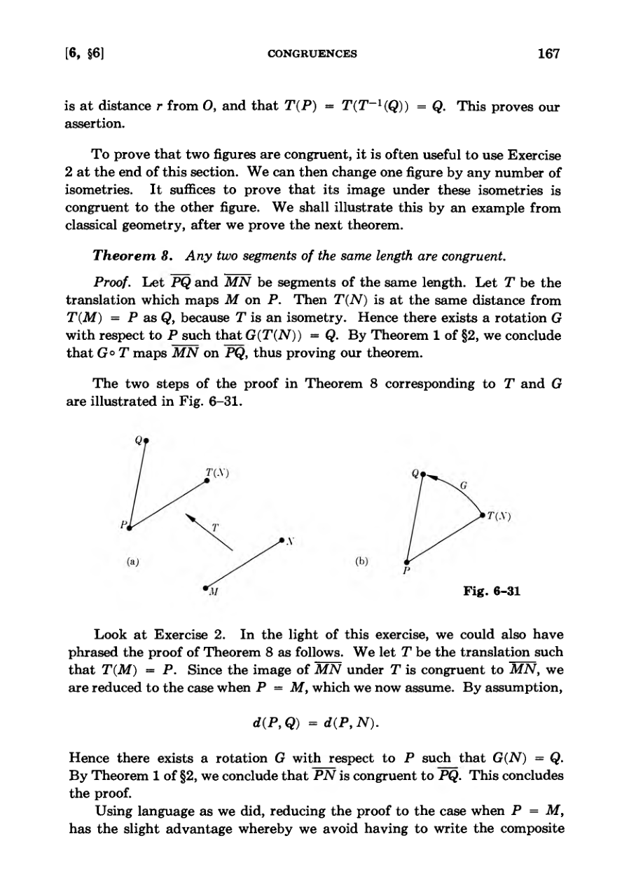
Theorem 8 proves that any two line segments of identical length are congruent using translations and rotations.
Proofs can be simplified by strategically reducing cases so that starting points coincide, avoiding complex composite assertions.
Theorem 9 establishes the congruence of right triangles with equal corresponding legs, connecting classical geometry to isometry principles.
Theorem 10 proves the general triangle congruence case where all three corresponding sides have equal lengths.
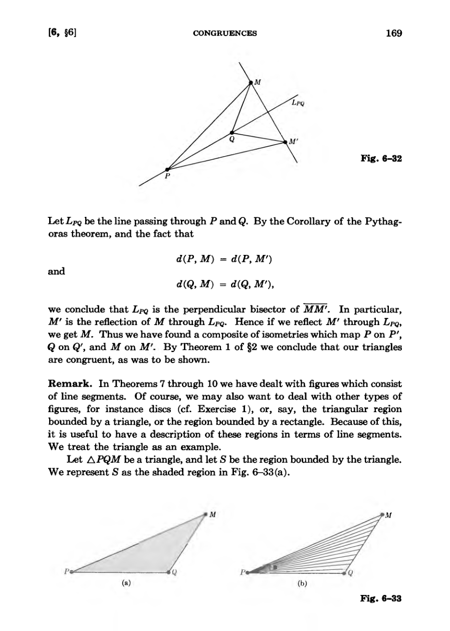
Reflections and perpendicular bisectors are utilized to map remaining points and complete the ultimate triangle congruence proof.
These methods extend beyond simple line segments to bounding regions like triangular surfaces and discs.
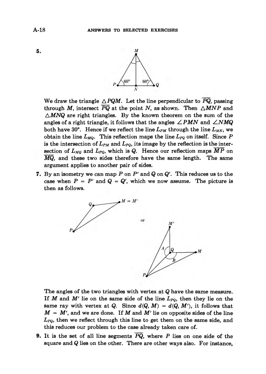
Hence if we reflect M' through Lpq, we get M.
FigureDiagram
Geometrical Shapes And Isometries
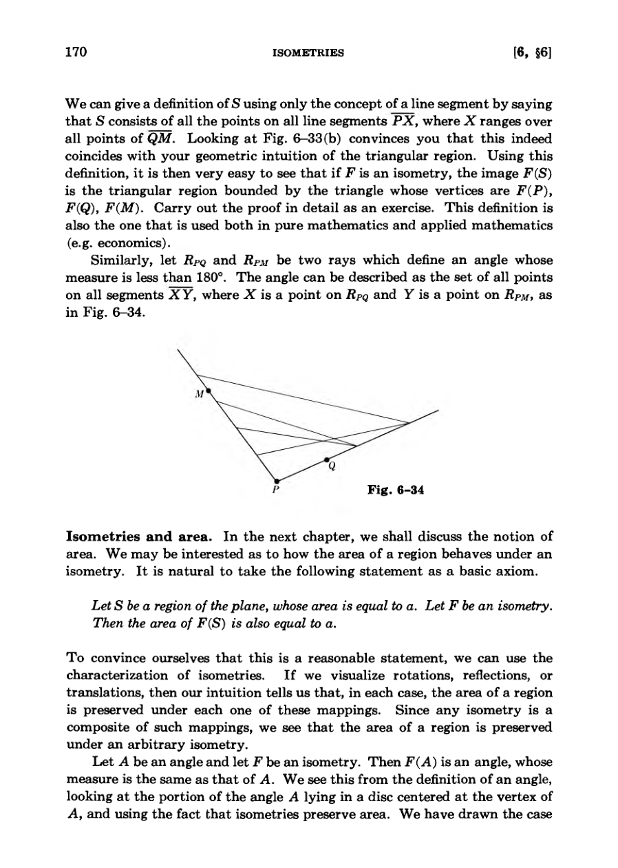
Geometric regions and angles can be formally defined using sets of line segments connecting points.
This foundational definition applies consistently across both pure mathematics and applied fields like economics.
Area preservation under isometries is established as a basic axiom, supported by visualizing basic mappings such as rotations and reflections.
Because any isometry is a composite of rotations, reflections, or translations, the area of any region remains unchanged under an arbitrary isometry.
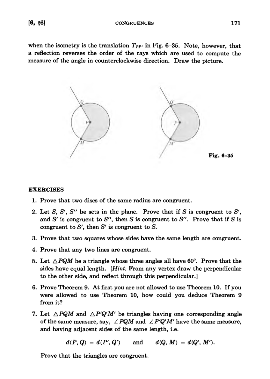
Isometries preserve the measure of angles, though reflections have the specific property of reversing the order of the rays used to compute that measure.
Note, however, that a reflection reverses the order of the rays which are used to compute the measure of the angle in counterclockwise direction.
DiagramFigureDiagram
Area and Dilation
We assume the basic intuitive properties of area, such as the area of a square being a squared and a rectangle being the product of its sides.
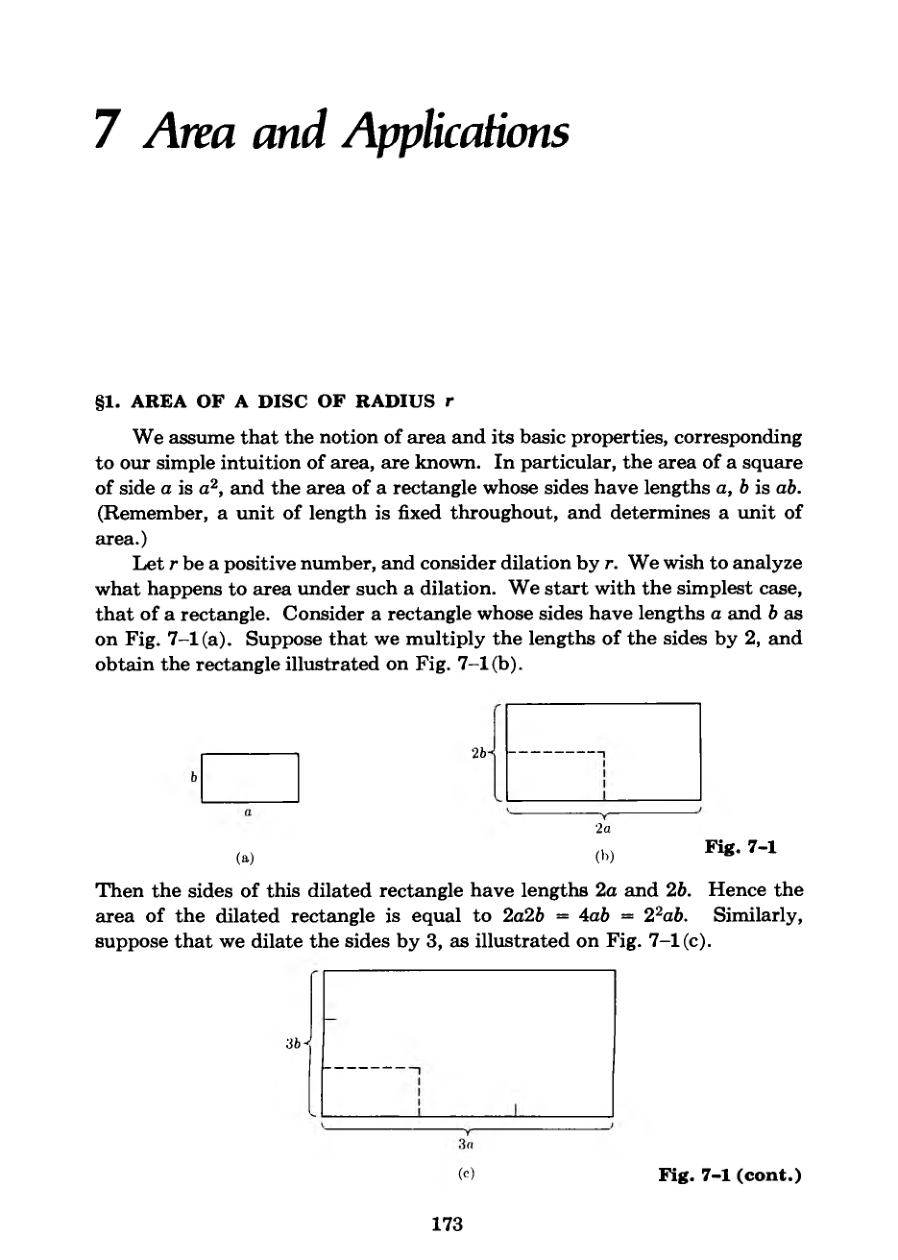
When a rectangle with sides a and b is dilated by a positive factor r, its new sides become ra and rb, resulting in an area of r squared times ab.
This establishes that the area of a rectangle changes by a factor of r squared under a dilation by r.
It is plausible that any arbitrary planar region approximated by rectangles will also have its area change by a factor of r squared under dilation.
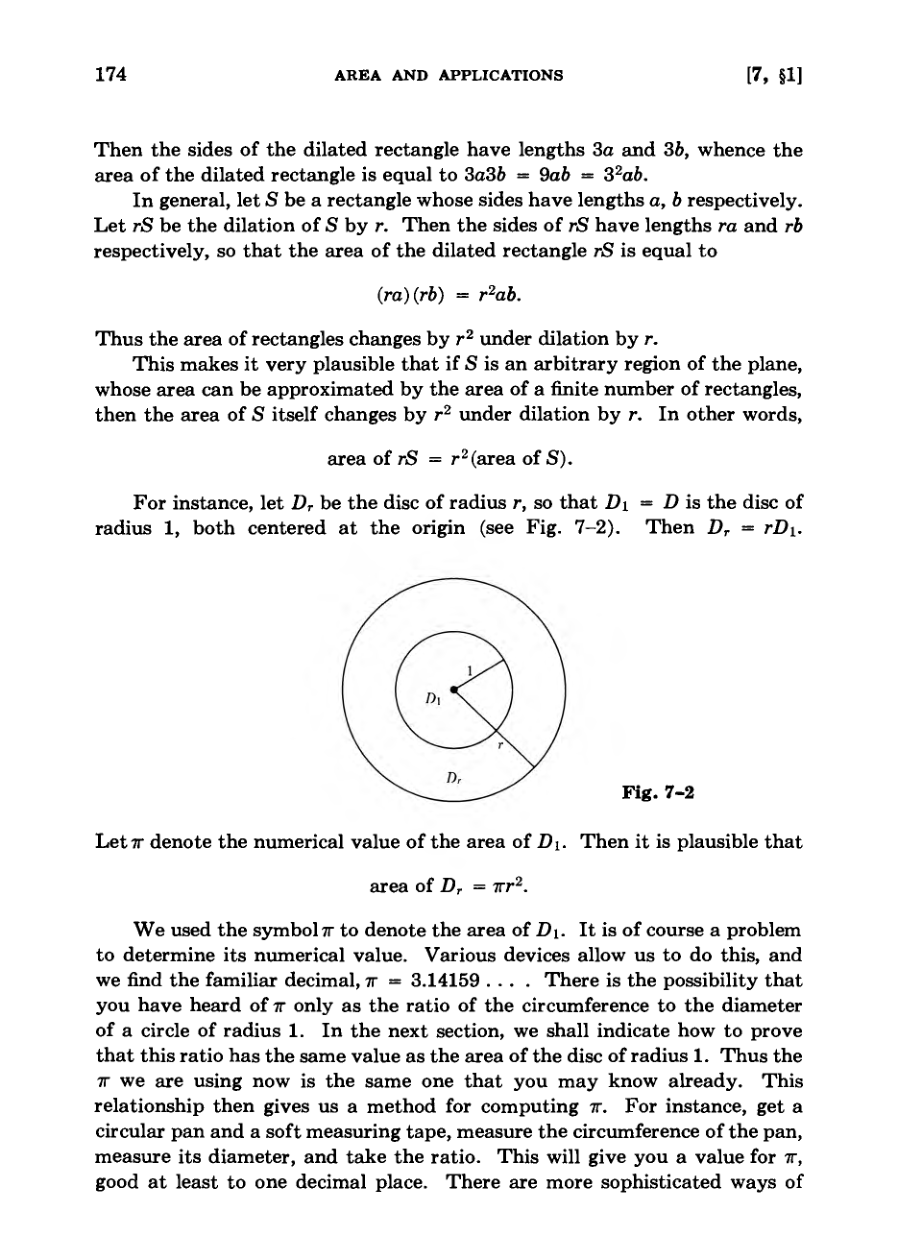
Using this principle, the area of a disc of radius r is expressed as pi times r squared, where pi represents the numerical area of a disc of radius one.
It is of course a problem to determine its numerical value.
DiagramDiagramFigureDiagram
Approximating Area with Grids
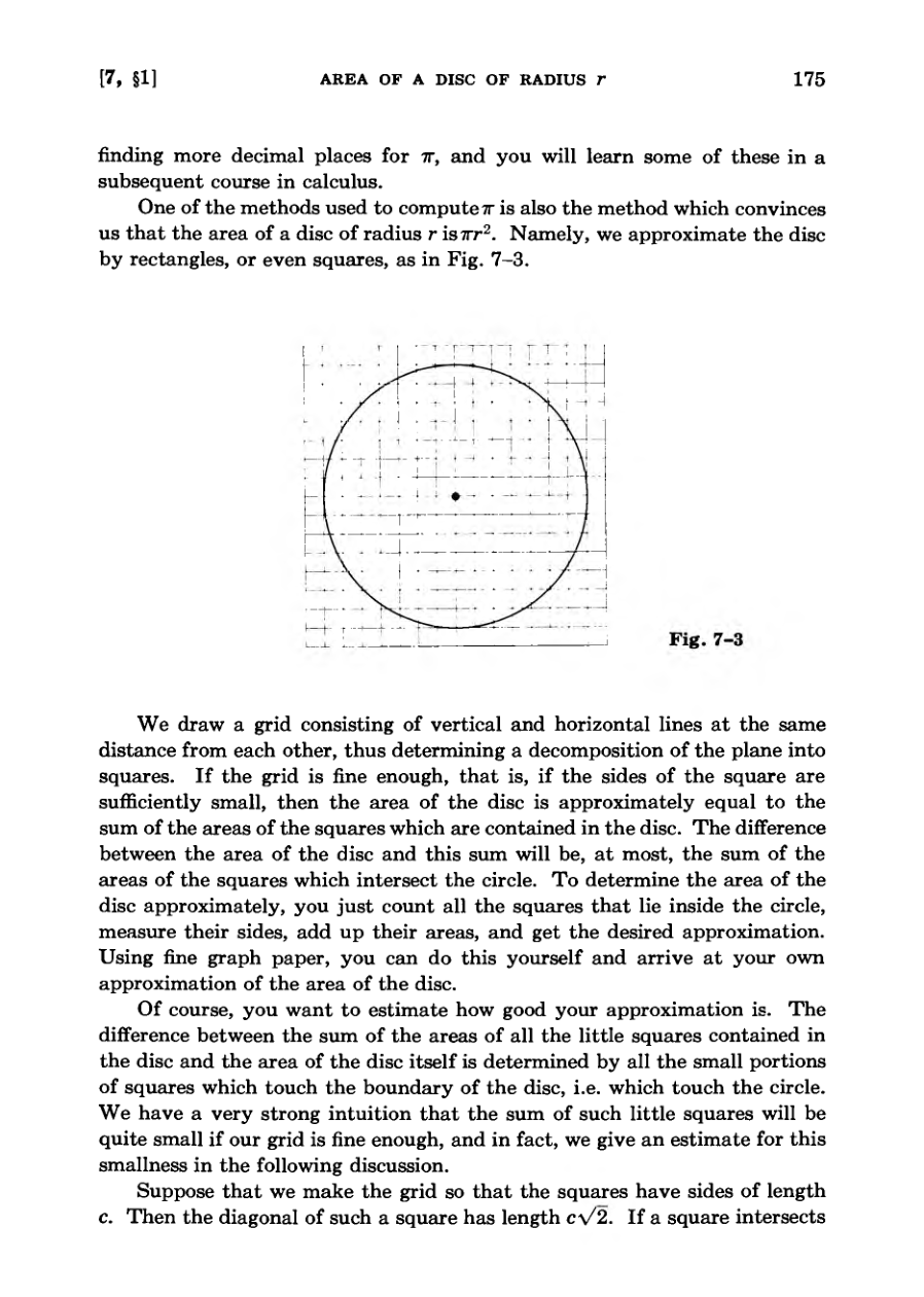
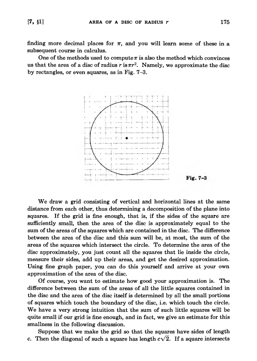
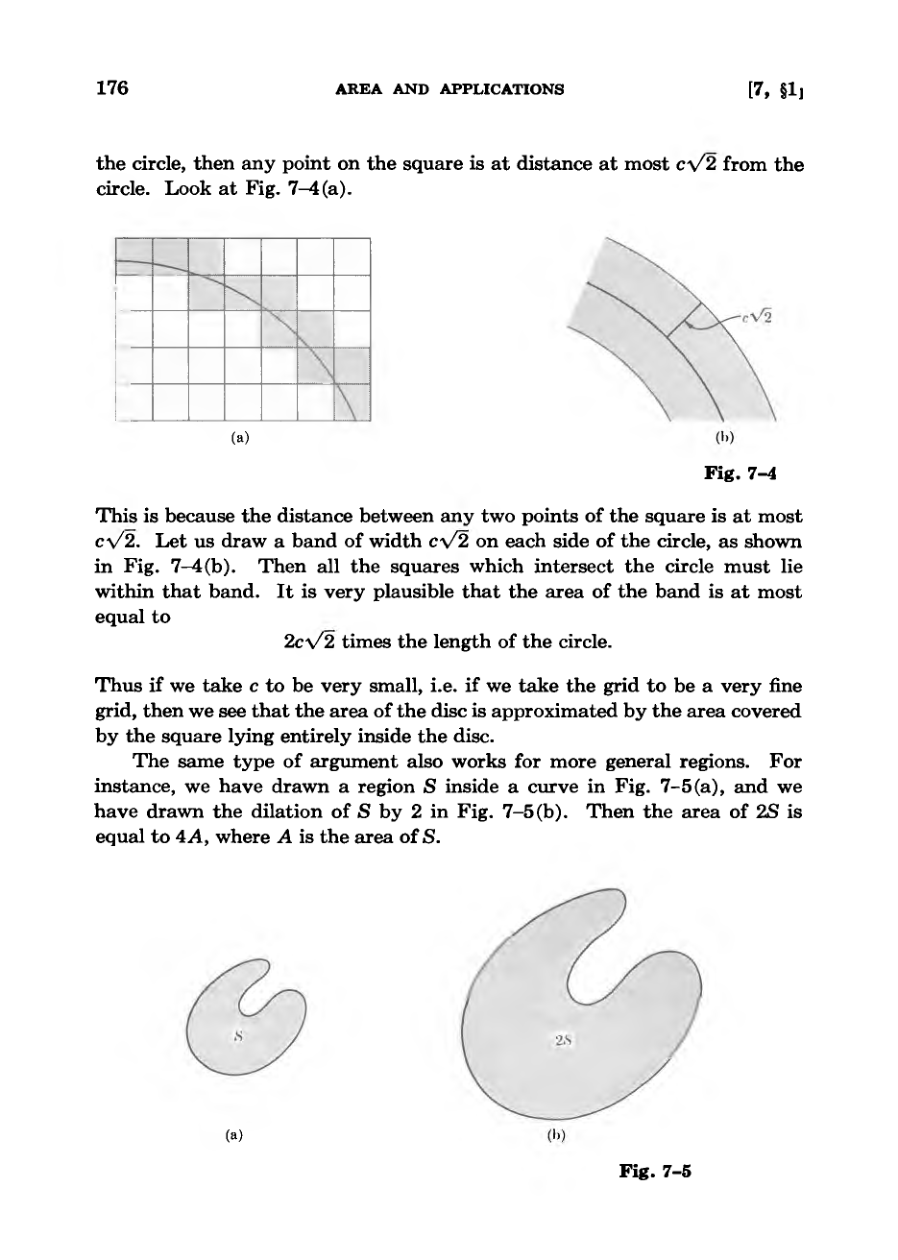
The area of a disc can be approximated by summing the areas of small grid squares contained within it.
The error of this approximation is bounded by the squares that intersect the boundary circle.
By making the grid finer, the total area of the boundary-touching squares becomes vanishingly small.
This grid-based approximation method can be generalized to apply to more complex regions and dilations.
We have a very strong intuition that the sum of such little squares will be quite small if our grid is fine enough, and in fact, we give an estimate for this smallness in the following discussion.
DiagramFigureFigure
Dilation and Circle Circumference
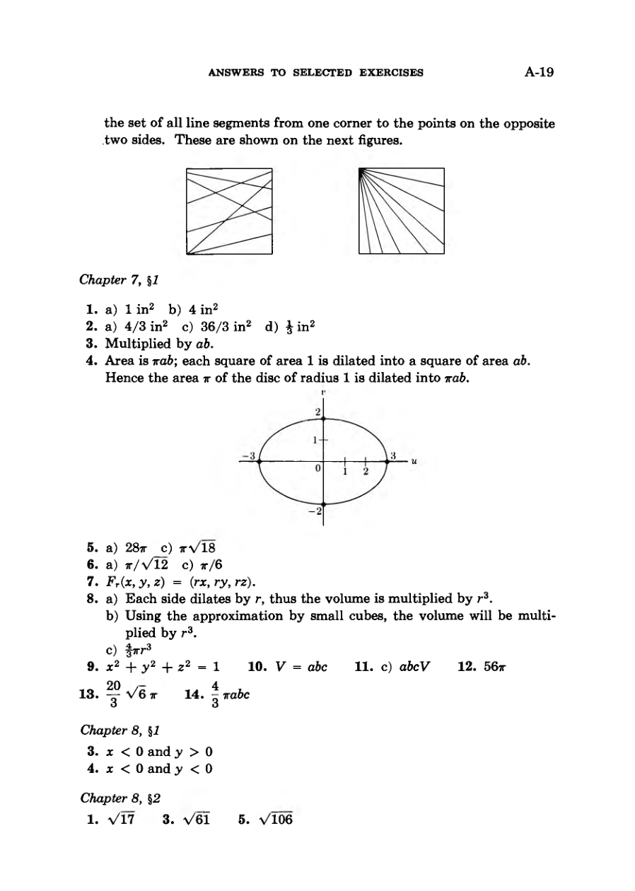
Mixed dilations stretch coordinate axes by factors like a, b, and c to transform geometric figures in two and three dimensions.
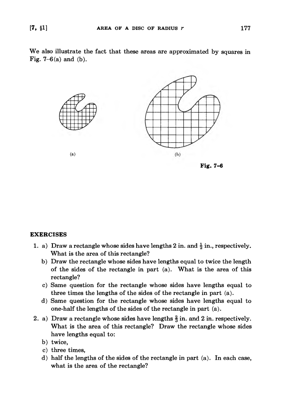
Exercises explore how volumes and areas change under these scaling transformations for rectangles, ellipses, and three-dimensional solids.
The text generalizes these scaling concepts from the plane to 3-space and speculates on n-dimensional spaces.
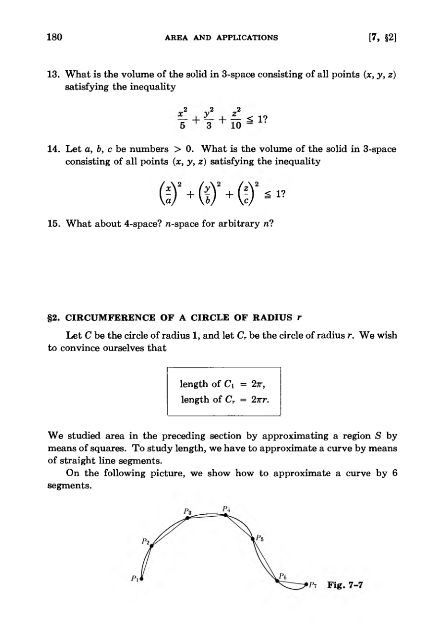
To study the length of a curve like a circle, the text transitions from approximating areas with squares to approximating curves with straight line segments.
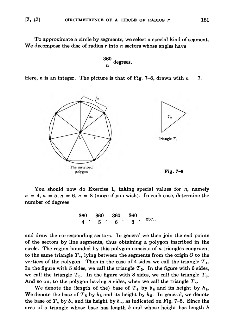
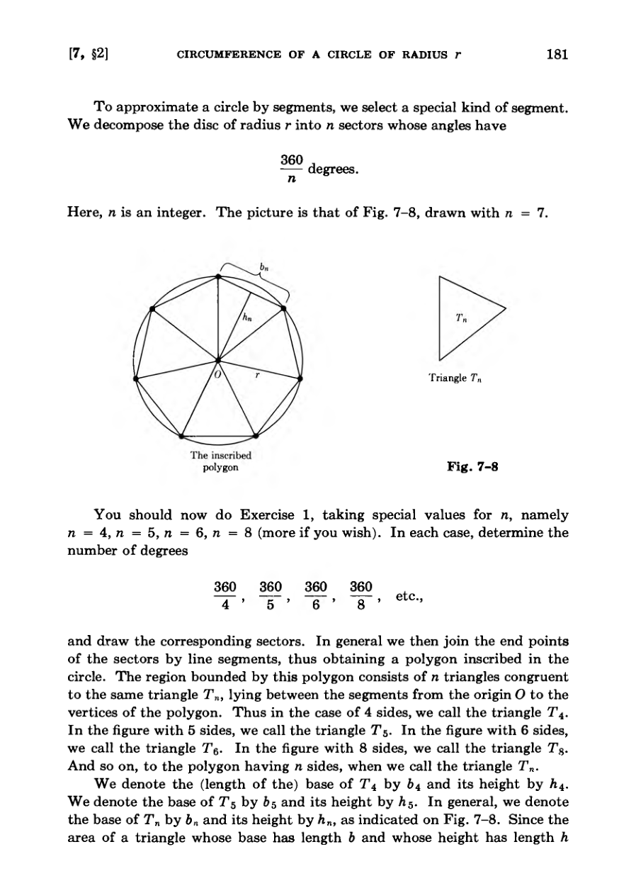
A circle of radius r is analyzed by decomposing a disc into n sectors to approximate its circumference as 2 pi r.
To study length, we have to approximate a curve by means of straight line segments.
DiagramDiagram
Circle Area and Dilation
Constructing inscribed polygons inside circles helps define and calculate the area and perimeter.
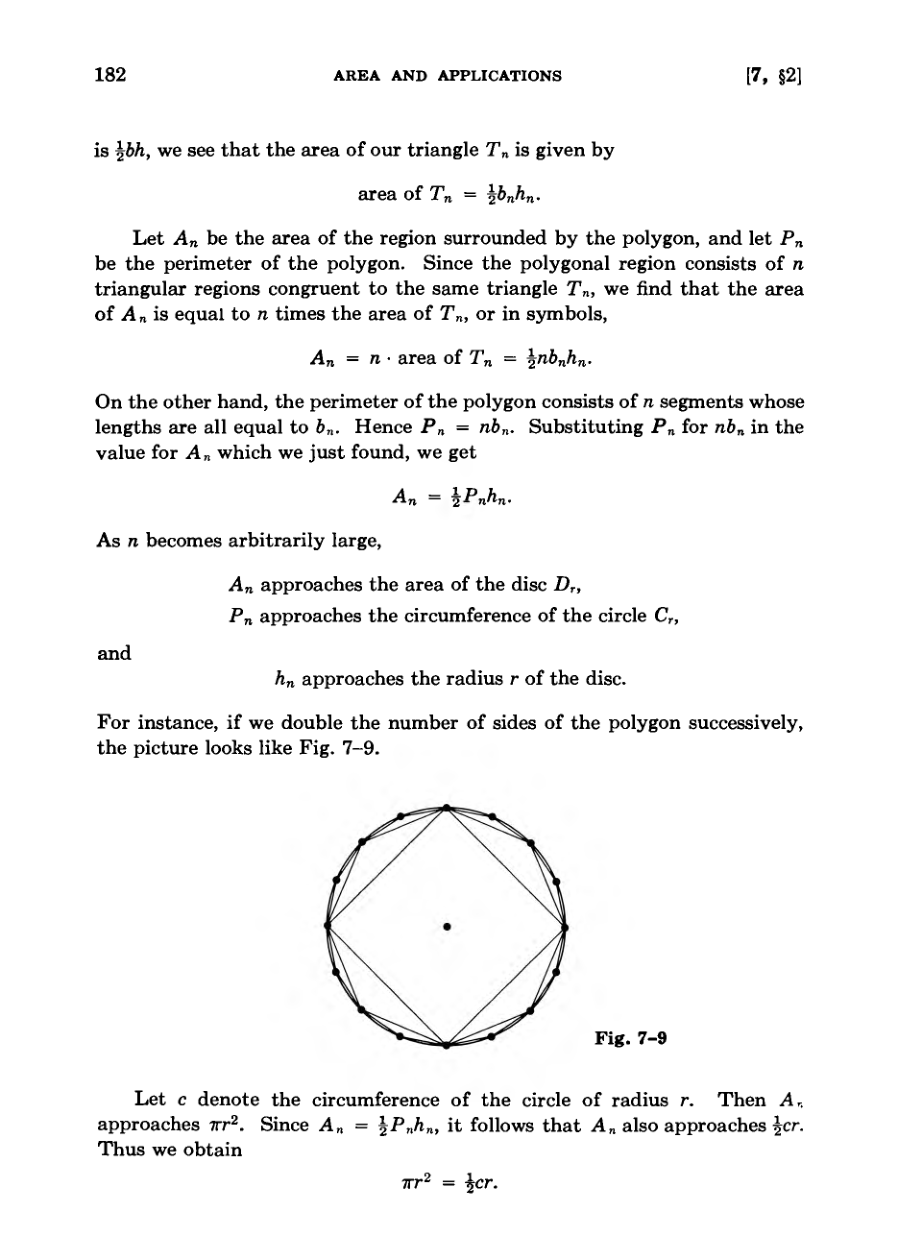
As the number of polygon sides increases, its area and perimeter approach the area and circumference of the circle.
By taking the limit as sides increase, the classic formula for the circumference of a circle is derived.
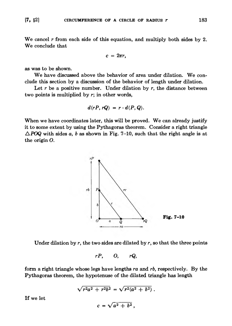
Dilation scales the distance between points and the lengths of triangle sides by a factor of r.
The length scaling property extends to arbitrary curves by approximating them with linear segments.
As n becomes arbitrarily large, An approaches the area of the disc Dr, Pn approaches the circumference of the circle Cr, and hn approaches the radius r of the disc.
DiagramFigureDiagram
Introduction to Coordinate Geometry
The text connects geometric scaling limits to the foundational concepts of calculus.
Practical exercises invite readers to empirically approximate pi using physical objects.
Part Three introduces coordinate geometry as a method to translate geometric terms into numerical properties.
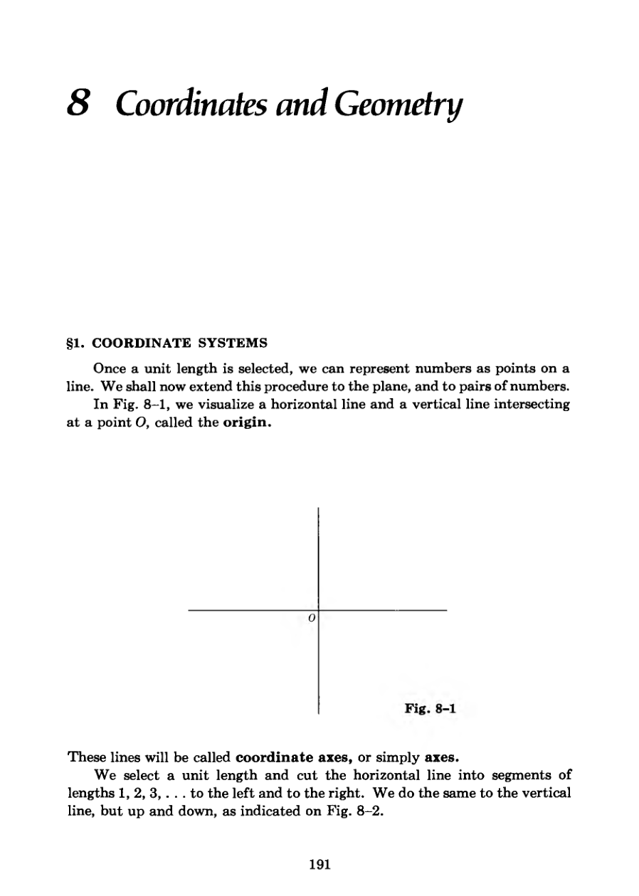
Coordinate systems extend the representation of numbers from a single line to pairs of numbers in a plane.
The intersection of coordinate axes at the origin forms the basis for analytical computation in geometry.
Giving coordinates to points not only allows us to give analytic proofs.
Diagram
Introduction to Coordinate Systems
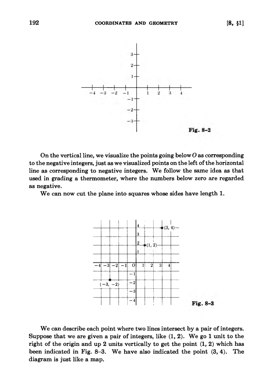
The plane can be divided into a grid using horizontal and vertical axes, analogous to a thermometer or a map.
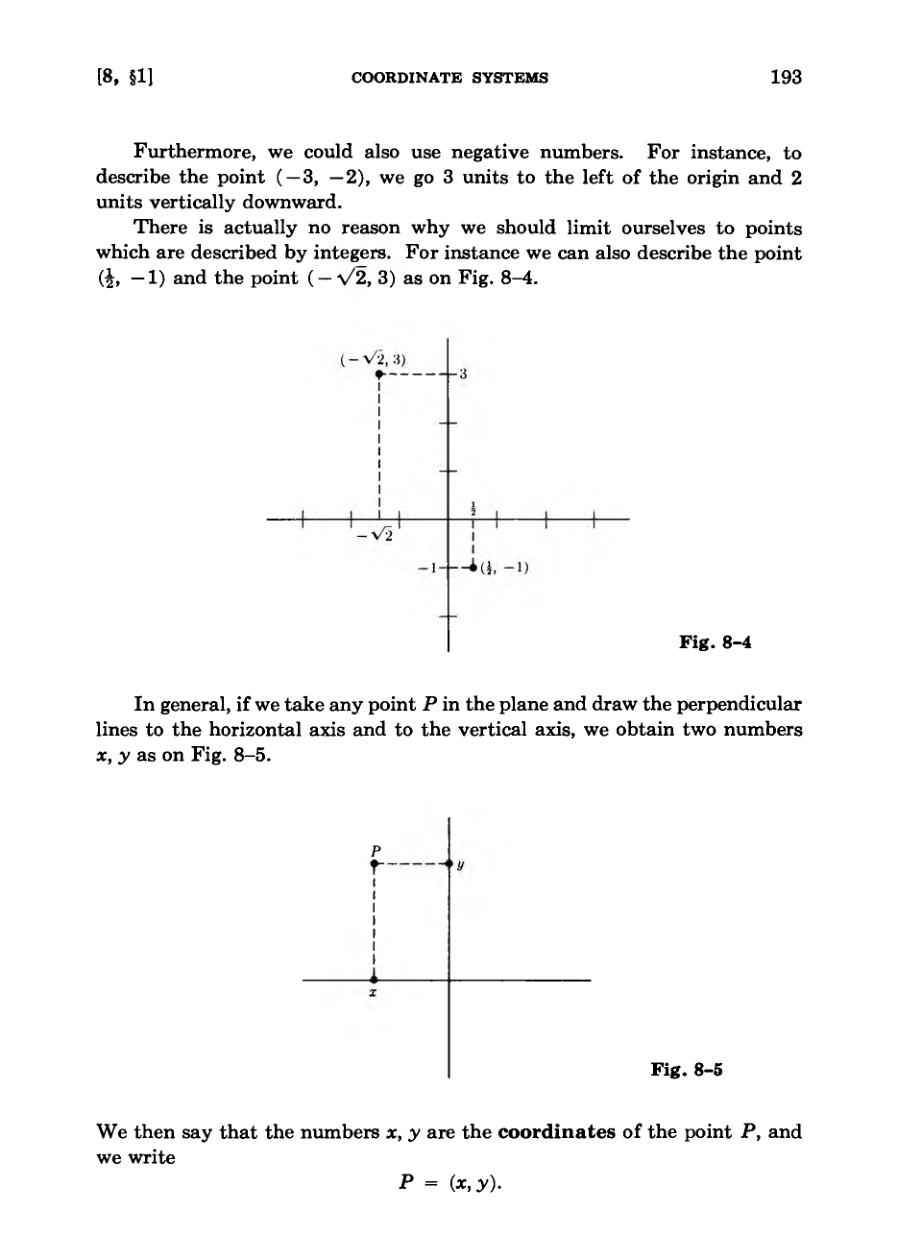
Points on the grid are identified using pairs of integers or numbers, such as positive and negative coordinates.
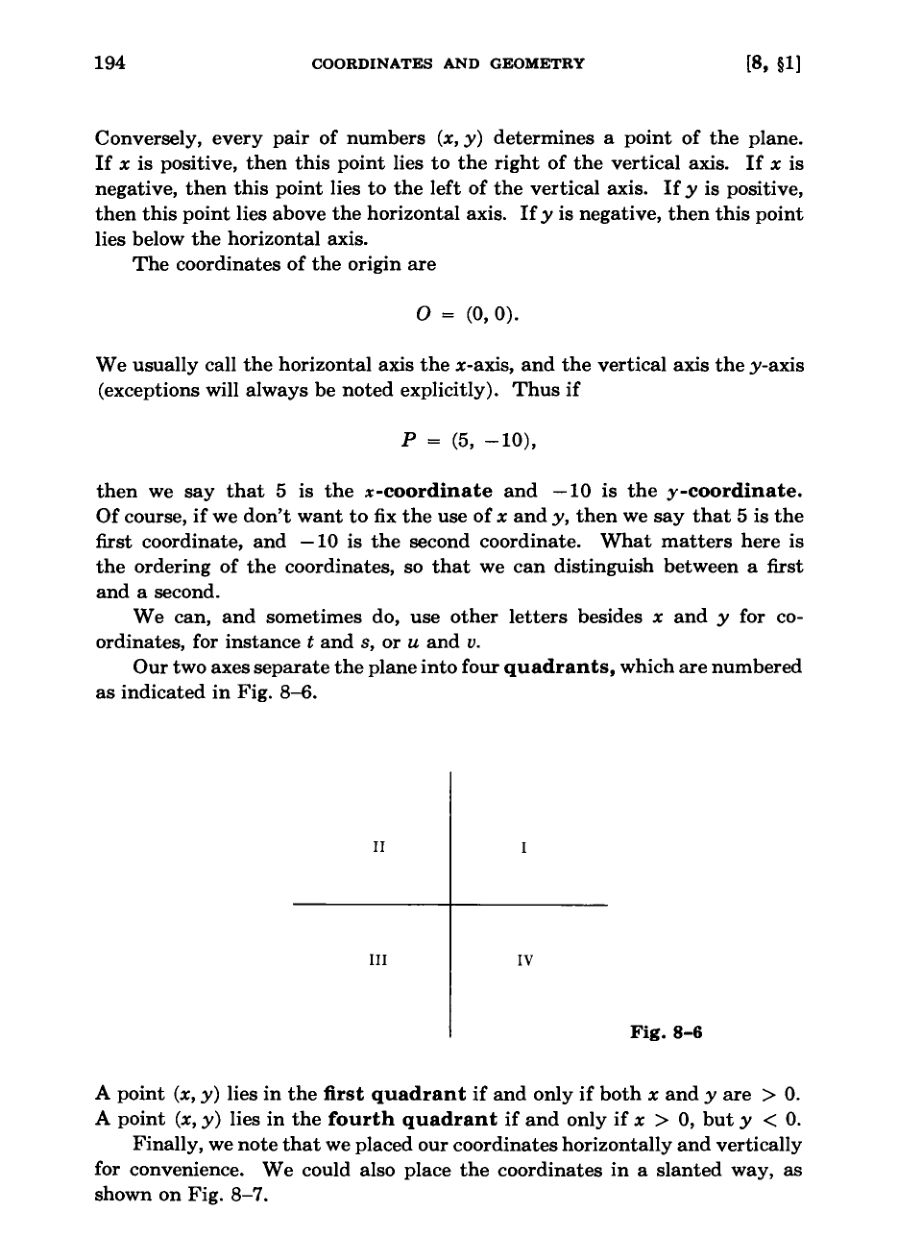
Every point P in the plane corresponds to a unique pair of numbers (x, y) known as its coordinates.
The two axes divide the plane into four distinct quadrants based on the signs of their x and y values.
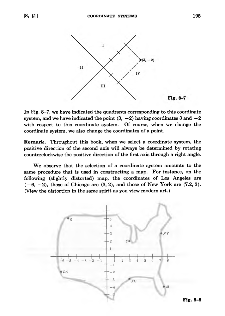
Coordinate systems are flexible and can even be represented using slanted axes or applied to map geographical locations.
View the distortion in the same spirit as you view modern art.
DiagramDiagramDiagramFigure
Coordinates and Distance Geometry
Exercises involve plotting various points on a coordinate plane and determining coordinates for geographic locations.
A continuous big exercise challenges students to extend two-dimensional geometric concepts into three-dimensional space.
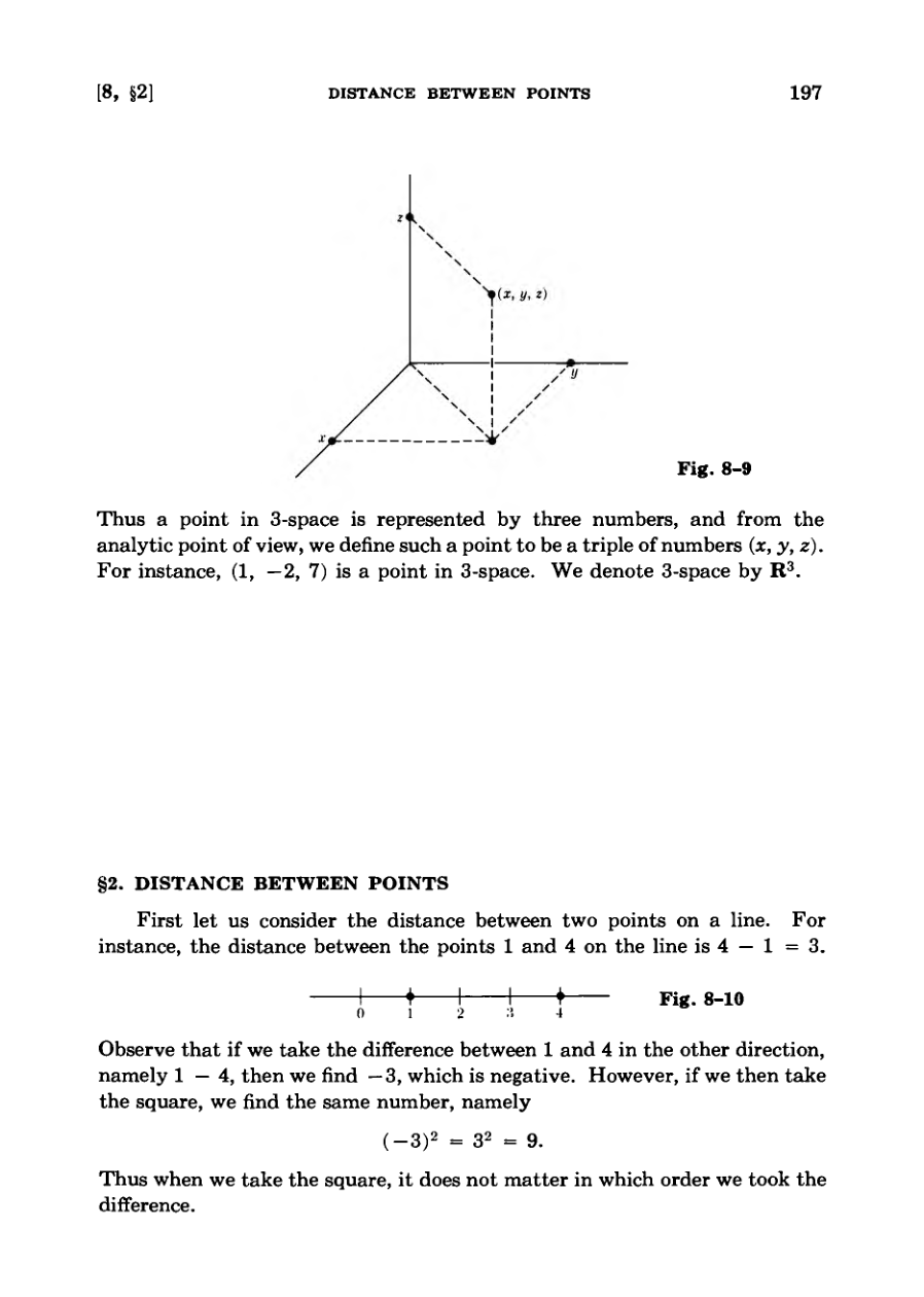
Points in three-dimensional space are defined analytically as a triple of numbers denoted as R3.
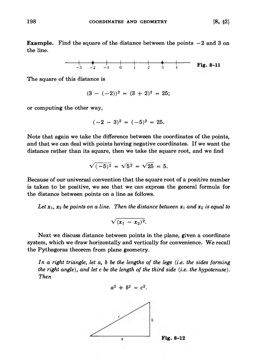
The distance between points on a line can be determined by squaring their coordinate differences and taking the square root.
Squaring the difference between points eliminates directional sign discrepancies in distance calculations.
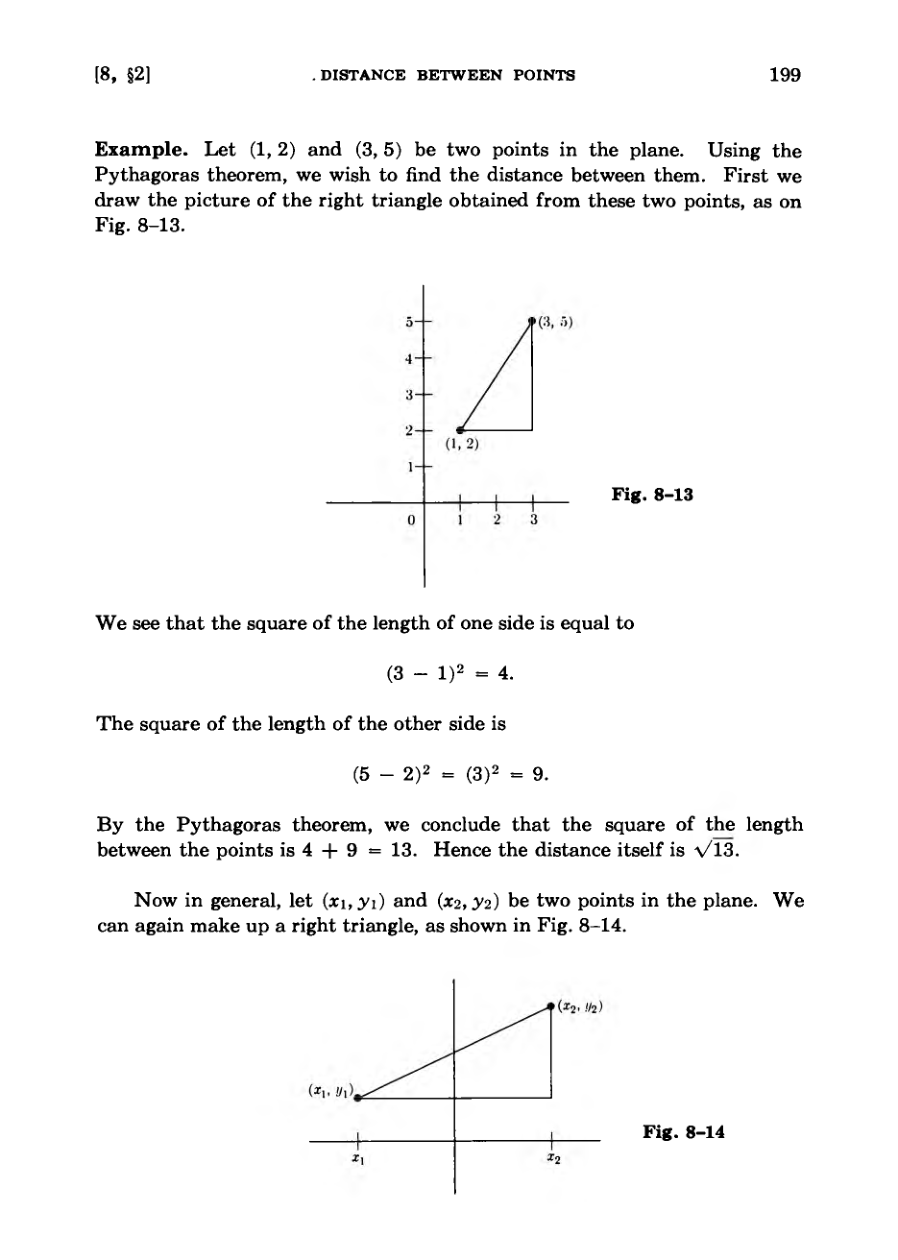
The text introduces the Pythagorean theorem to calculate distances between points in a two-dimensional plane.
Write it all up as if you were writing a book. This will make you really learn the subject.
DiagramDiagram
Distance Between Points
The Pythagoras theorem is used to determine the distance between two points in a plane.
A general distance formula is derived using the coordinates of any two points.
Computing distance yields the same result regardless of the order in which the points are chosen.
The plane is formally defined as the set of all pairs of real numbers to build geometry upon number properties.
The distance concept can be extended to three-dimensional space using a generalized Pythagorean formula.
Warning: Always be careful when you meet minus signs.
Diagram
The Equation of a Circle
Distance formulas in 3-space can be justified geometrically using the Pythagorean theorem in horizontal and vertical planes.
Scaling a point by a positive number r multiplies the distance between points by the same factor r.
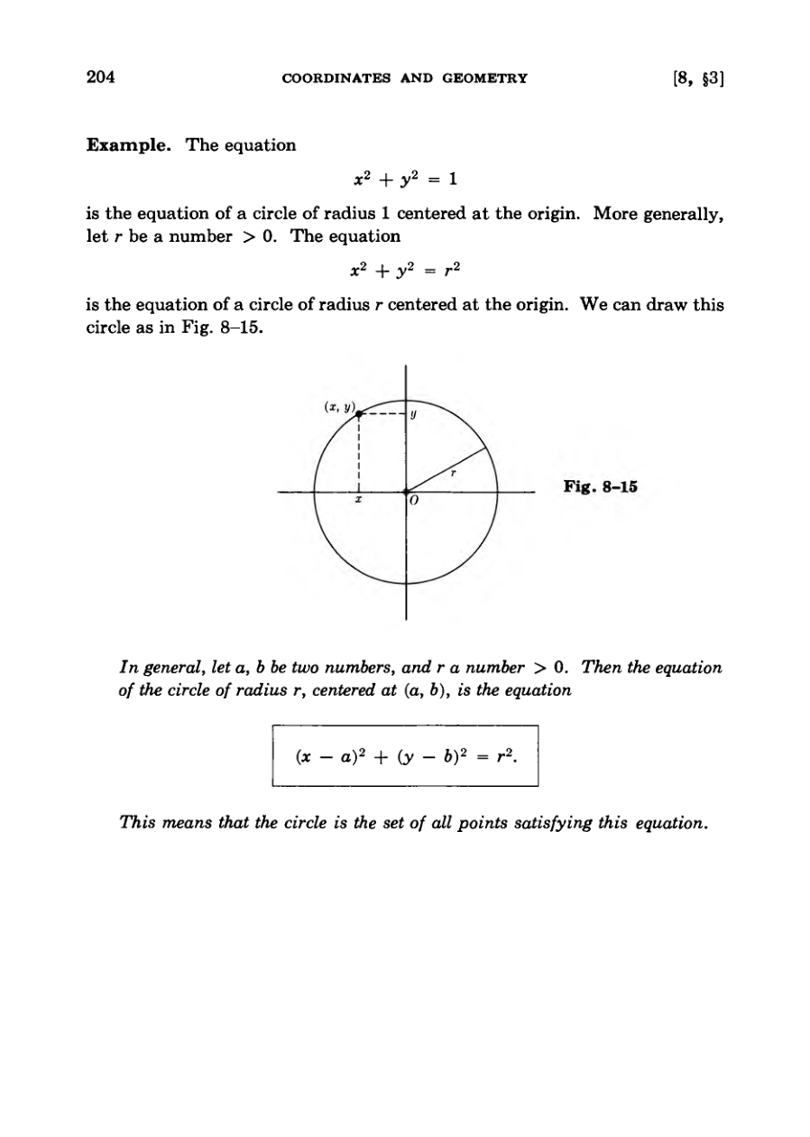
A circle is formally defined as the set of all points maintaining a fixed distance r from a given center point P.
The algebraic equation of a circle in coordinates can be derived directly by applying the distance formula.
Squaring both sides of the distance equation helps avoid messy square root signs in standard circle equations.
The general equation for a circle centered at point (a, b) with radius r is given by (x - a) squared plus (y - b) squared equals r squared.
It is often convenient to leave the equation of the circle in the form, to avoid writing the messy square root sign.
Diagram
Rational Points On Circles
The text introduces geometric exercises involving equations of spheres in 3-space, focusing on finding centers and radii.
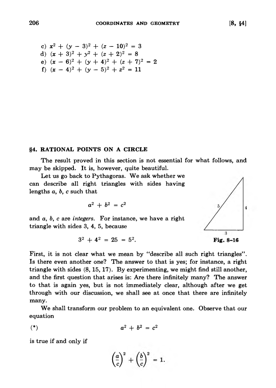
It transitions into the study of rational points on a circle and Pythagorean triples, asking if there are infinitely many integer solutions to a squared plus b squared equals c squared.
By dividing the equation by c squared, the problem of finding integer right triangles is transformed into finding rational points on the unit circle.
A rational point is defined as a point where both coordinates x and y are rational numbers.
The text demonstrates how assigning rational values to a parameter t generates coordinates on the unit circle, which recover known Pythagorean triples like (3, 4, 5) and (8, 15, 17).
The result proved in this section is not essential for what follows, and may be skipped. It is, however, quite beautiful.
Diagram
Rational Points On Circles
Formulas involving a parameter t generate rational points on a circle and right triangles with integral sides.
Mathematical talent is distinguished by the ability to discover such beautiful formulas rather than merely plugging numbers into them.
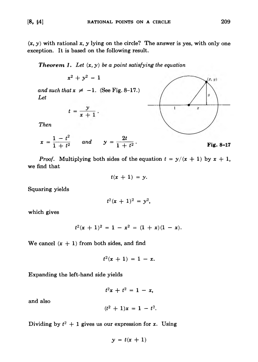
Theorem 1 proves that almost all rational points on a unit circle can be expressed using rational values of t.
Extending this inquiry to higher powers leads to Fermat's equation and the famous unresolved problems surrounding it.
What distinguishes someone with talent for mathematics from someone without talent is that the first person will be able to discover such beautiful formulas and the second person will not.
Diagram
Dilations and Reflections of Points
Points in the plane are represented as pairs of real numbers in a fixed coordinate system.
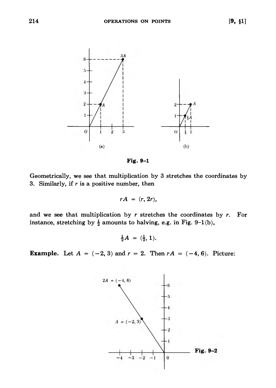
Multiplying a point by a real number scales its coordinates by that factor, a geometric process known as dilation.
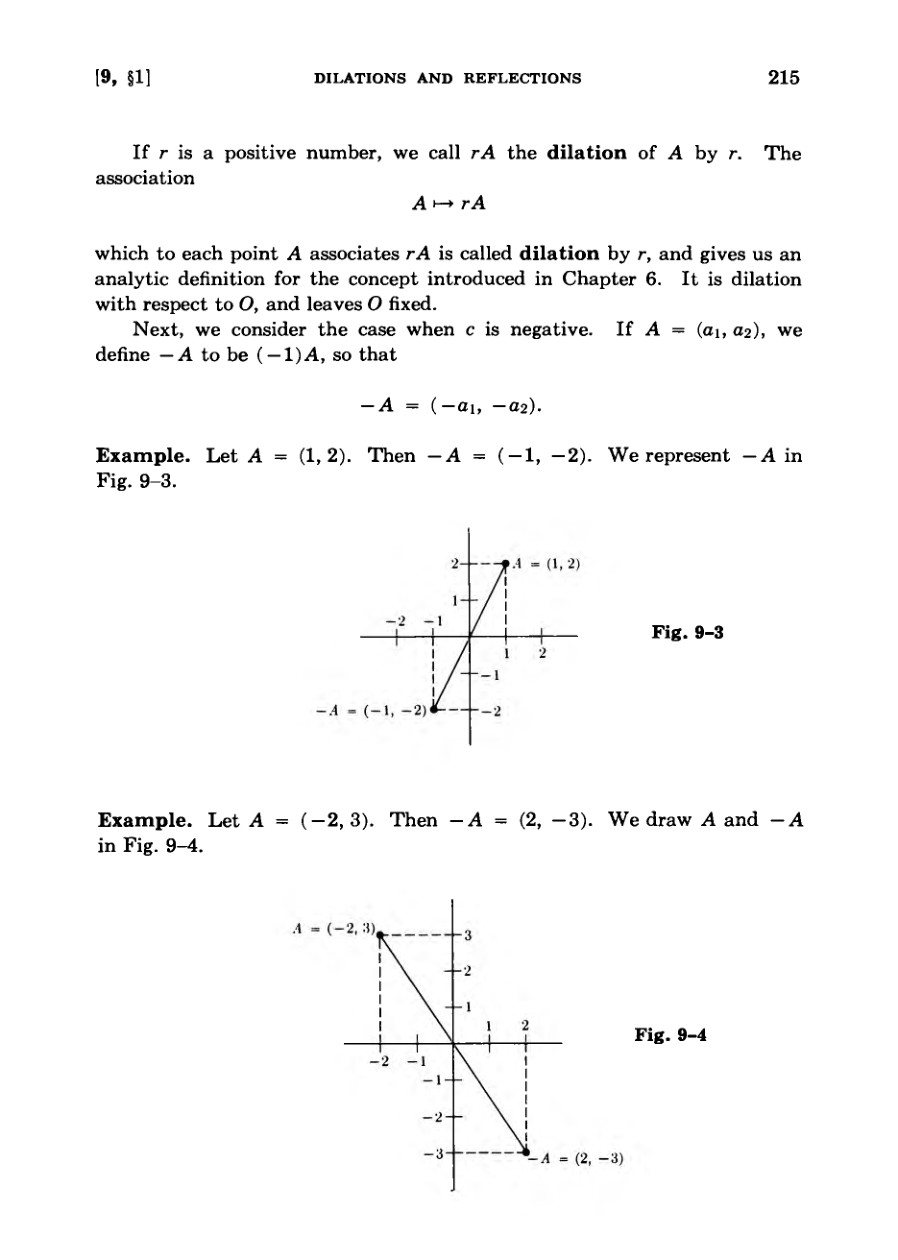
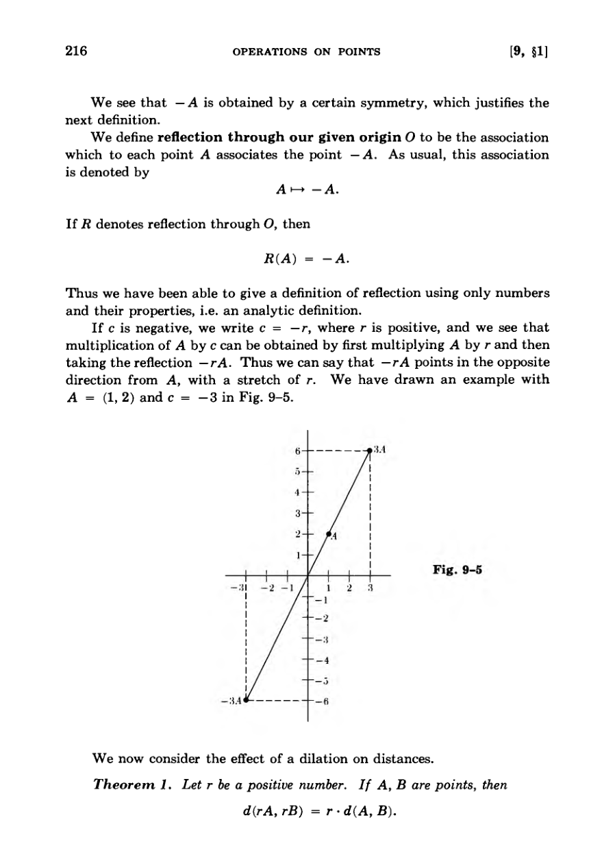
Multiplying a point by a negative number reverses its direction and scales it by the absolute value.
Reflection through the origin maps each point A to its negative counterpart -A.
Dilation by a positive factor r scales the distance between any two points by that exact same factor r.
Geometrically, we see that multiplication by 3 stretches the coordinates by 3.
DiagramFigureDiagram
Operations on Points
The text introduces exercises involving scalar multiplication of points and distance preservation under reflection.
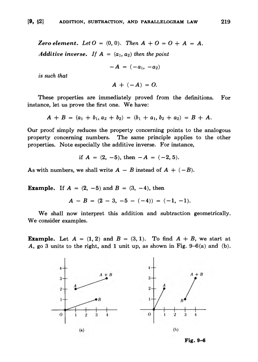
Point addition is defined componentwise, mirroring the properties of basic number addition such as commutativity and associativity.
Every point features an additive inverse, allowing subtraction of points to be defined consistently.
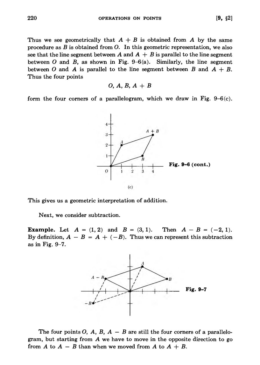
Geometric interpretation reveals that points O, A, B, and A + B form the corners of a parallelogram.
Subtraction of points is similarly represented using the additive inverse, maintaining the parallelogram geometric structure.
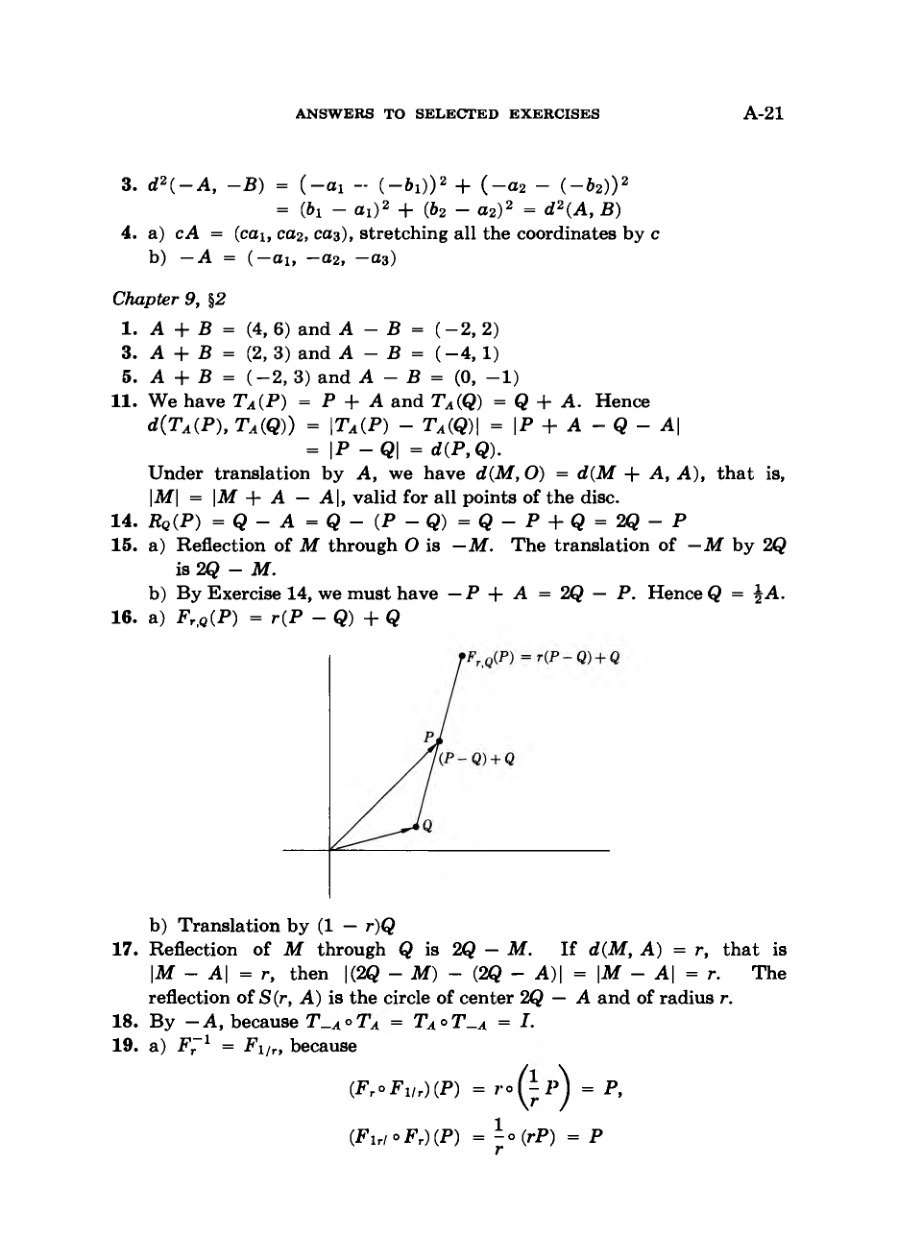
Thus the four points O, Ay By A + B form the four corners of a parallelogram, which we draw in Fig. 9-6 (c).
FigureDiagramDiagram
Geometric Translations and Norms
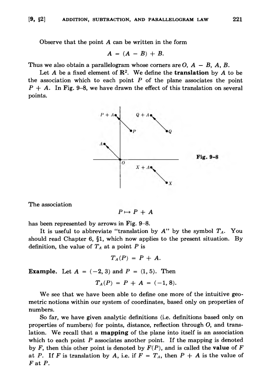
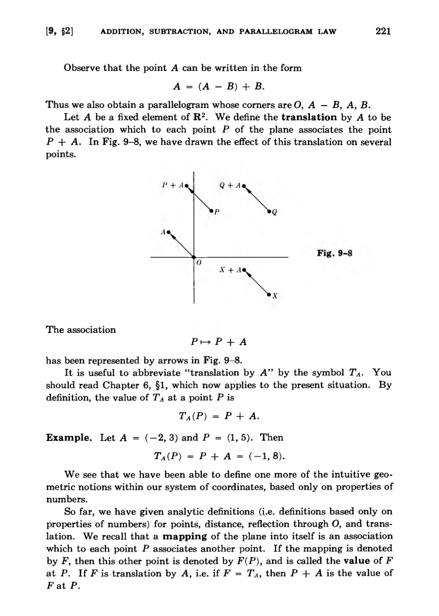
Translation by a vector A is defined analytically as the association mapping each point P to P plus A.
Geometric notions like distance and translation are successfully expressed using purely numerical properties.
An isometry is formally defined as a mapping of the plane into itself that preserves distances between points.
The distance between any two points A and B can be expressed neatly using the norm of their difference.
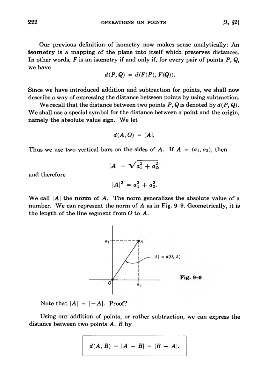
The norm of a point generalizes absolute value and represents the geometric length of the line segment from the origin.
We see that we have been able to define one more of the intuitive geometric notions within our system of coordinates, based only on properties of numbers.
DiagramDiagram
Operations and Transformations on Points
Points on any circle of radius r centered at A can be proven as images of points on a circle centered at O under translation.
Ordinary arithmetic rules for numbers, such as associativity and distributivity, apply directly to the addition and multiplication of points.
Proofs for point operations can be readily derived by reducing each statement to the analogous algebraic properties for numbers.
The provided exercises require plotting points, constructing parallelograms, and exploring geometric transformations.
Advanced exercises ask students to prove that translations are isometries and to analyze reflections and dilations in terms of transformations.
We ask whether the ordinary rules which we had for numbers also apply, and the answer is yes.
Mapping Exercises and 3-Space
Defines inverse mappings to prepare for geometric transformation exercises.
Explores properties of translations, dilations, and reflections through specific proofs.
Investigates basic unit points and coordinates, applying them to square and rectangle geometry.
Examines how geometric areas and lengths change under scaling and dilation.
Extends 2-dimensional concepts of points, translations, and isometries into 3-space and higher dimensions.
And higher. Why not?
Writing Mathematics and Segments
Mathematical training requires writing in full English sentences to force clear thinking.
Copying mathematical theory between dimensions or from experts is a historically valid learning technique, akin to Bach copying Vivaldi.
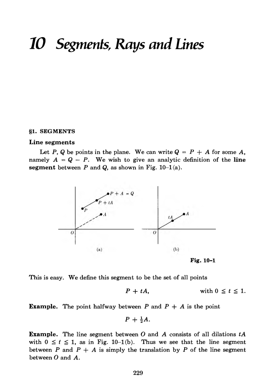
A line segment between points P and Q is defined analytically using the parameter t from 0 to 1.
The symmetry of line segments demonstrates that the segment between P and Q equals the segment between Q and P.
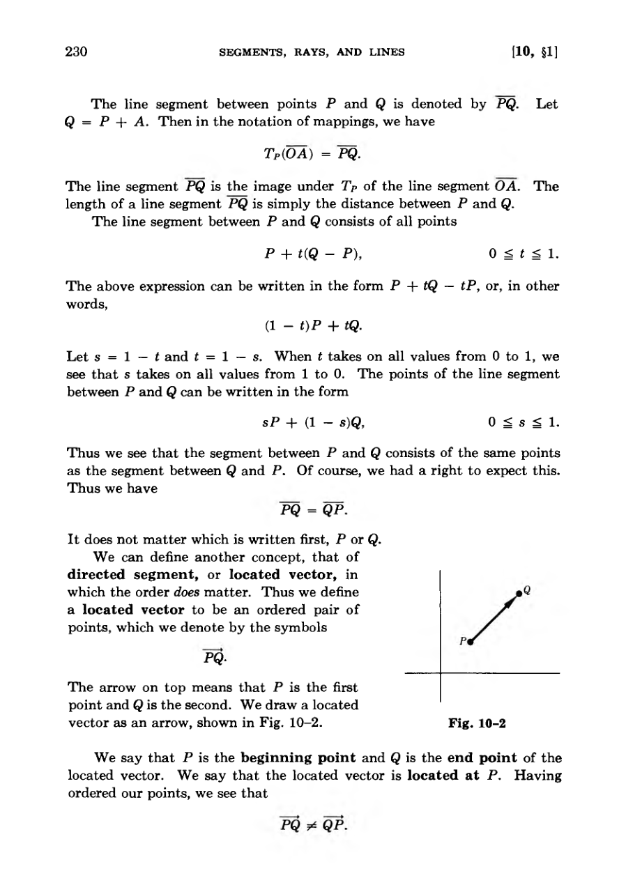
Directed segments or located vectors introduce an ordered pair of points where the direction and order matter.
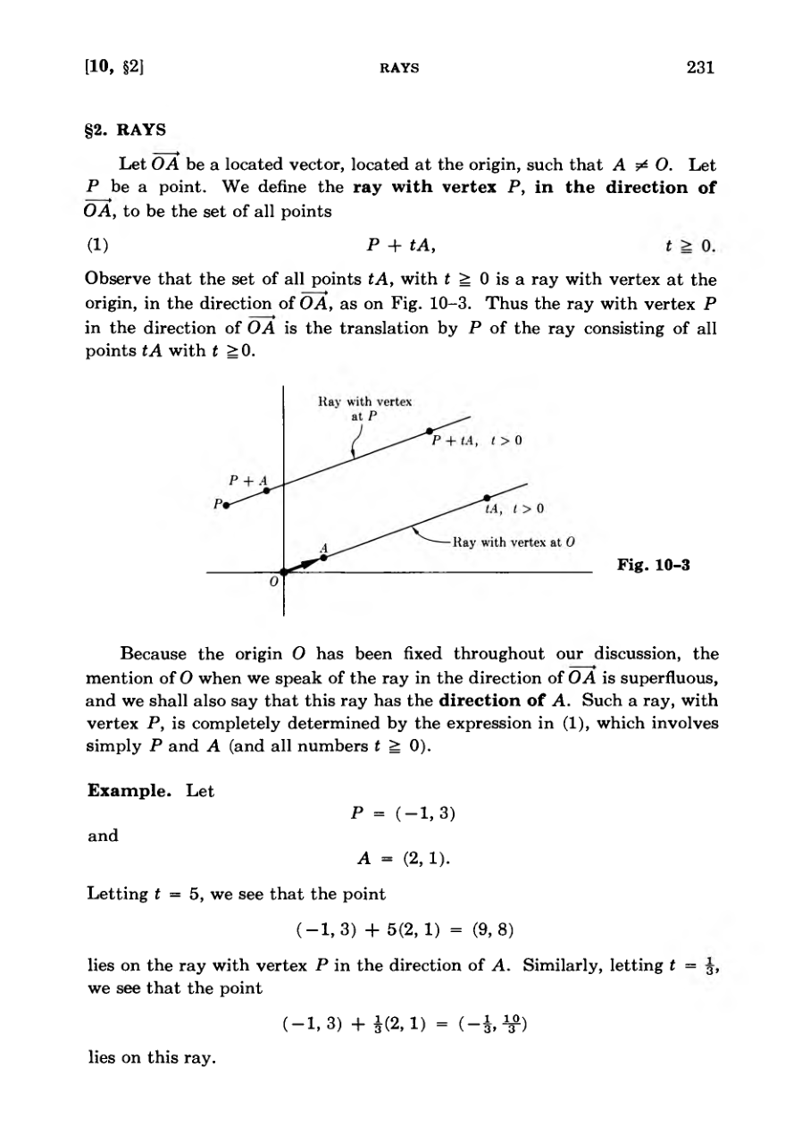
Rays are defined as sets of points extending infinitely in a specific direction from a vertex P using non-negative multipliers.
Do you know one of the means Bach used to learn how to compose? He copied practically the entire works of Vivaldi.
DiagramFigureDiagramFigure
Understanding Rays and Directions
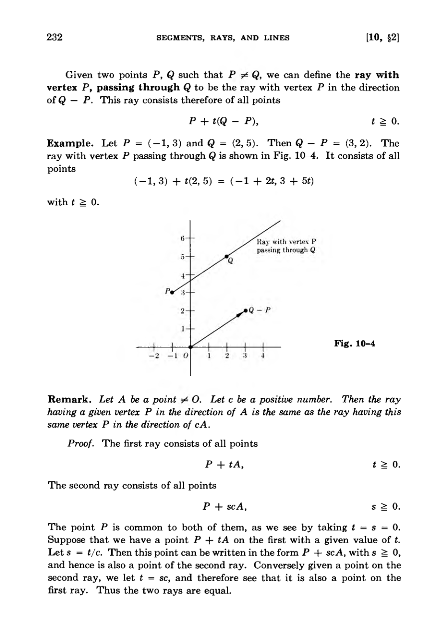
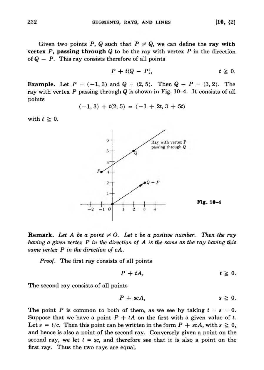
A ray starting at vertex P and passing through Q is defined algebraically using a parameter t greater than or equal to zero.
Scaling a direction vector by a positive number yields an identical ray originating from the same vertex.
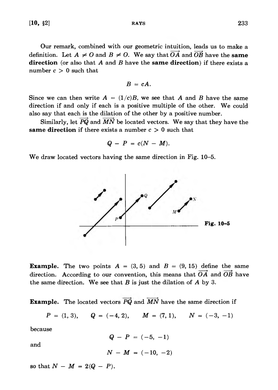
Two vectors or points are defined as sharing the same direction if one is a positive scalar multiple of the other.
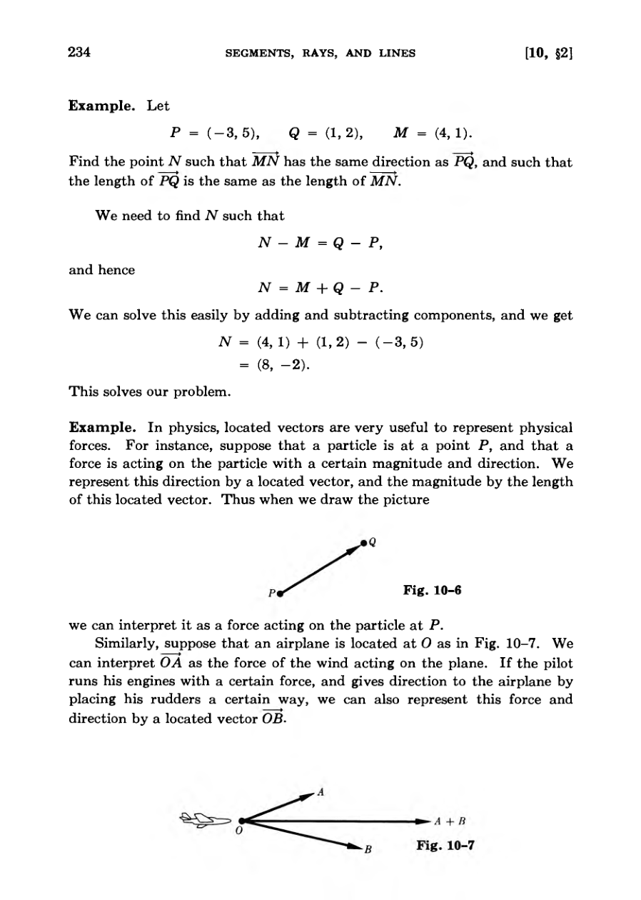
Located vectors can represent physical phenomena such as forces acting on particles or wind acting on airplanes.
Vector addition accurately models the combined movement resulting from multiple simultaneous physical forces acting on an object.
In physics, located vectors are very useful to represent physical forces.
FigureDiagramFigure
Vectors and Lines in Space
Exercises involve finding specific points along line segments defined by coordinates in both two and three dimensions.
Geometric mappings like translations and reflections are tested for preserving segments and rays.
Parallelism for located vectors is defined analytically using scalar multiples.
Transitive properties of parallel segments are assigned as proofs.
Lines passing through the origin are defined algebraically using scalar multiples of a point.
Let PQ and MN be located vectors such that P != Q and M != N.
Diagram
Parametric Representation of Lines
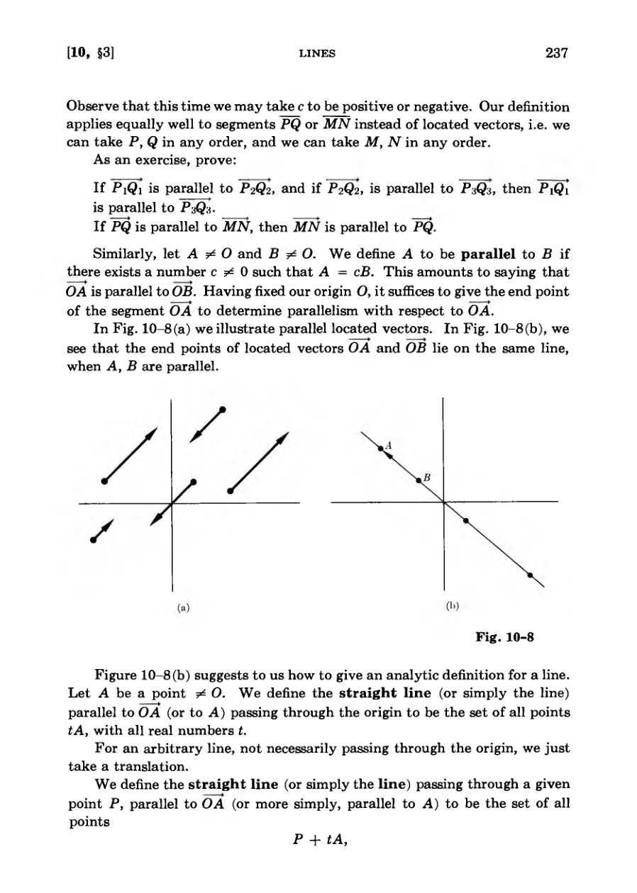
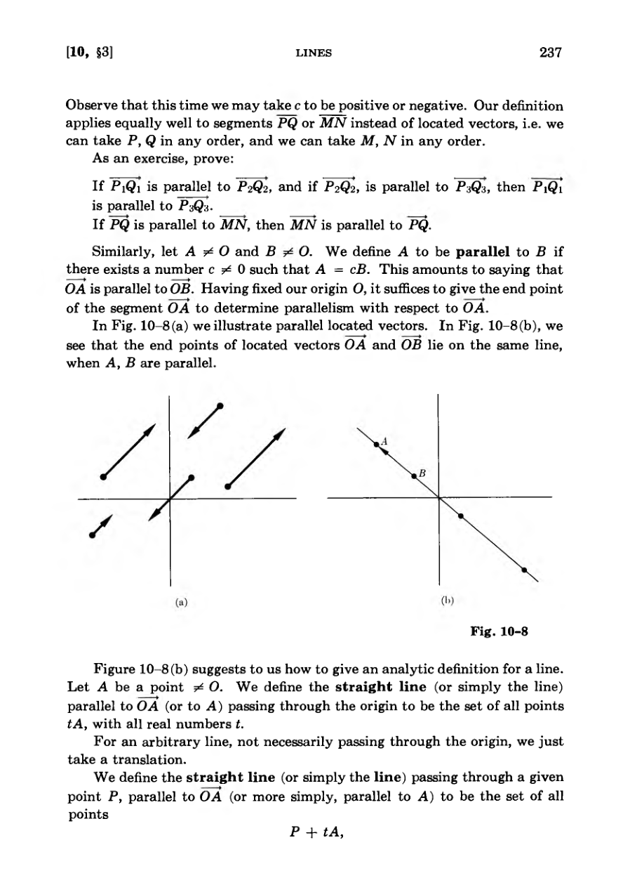
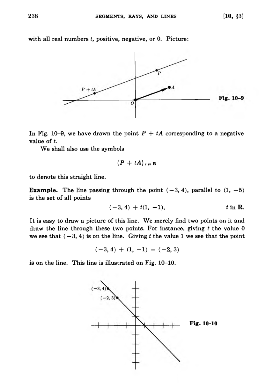
A straight line can be defined parametrically as the set of all points given by the formula P + tA for any real number t.
The parameter t can be interpreted physically as time, representing the position of a moving particle or bug along the line.
Parametric representations are advantageous because they generalize easily to three-dimensional space and capture uniform motion.
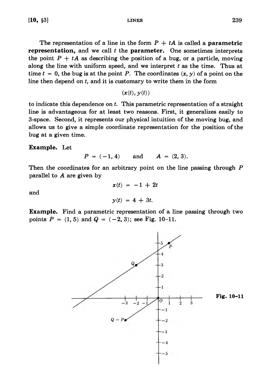
A line passing through two specific points P and Q can be parameterized using A = Q - P.
The velocity of a moving object is represented by the vector A, where its length corresponds to the speed of movement.
One sometimes interprets the point P + tA as describing the position of a bug, or a particle, moving along the line with uniform speed, and we interpret t as the time.
DiagramDiagramFigure
Intersections of Lines
Finding the intersection of two lines involves setting up a system of equations in two unknowns and solving them.
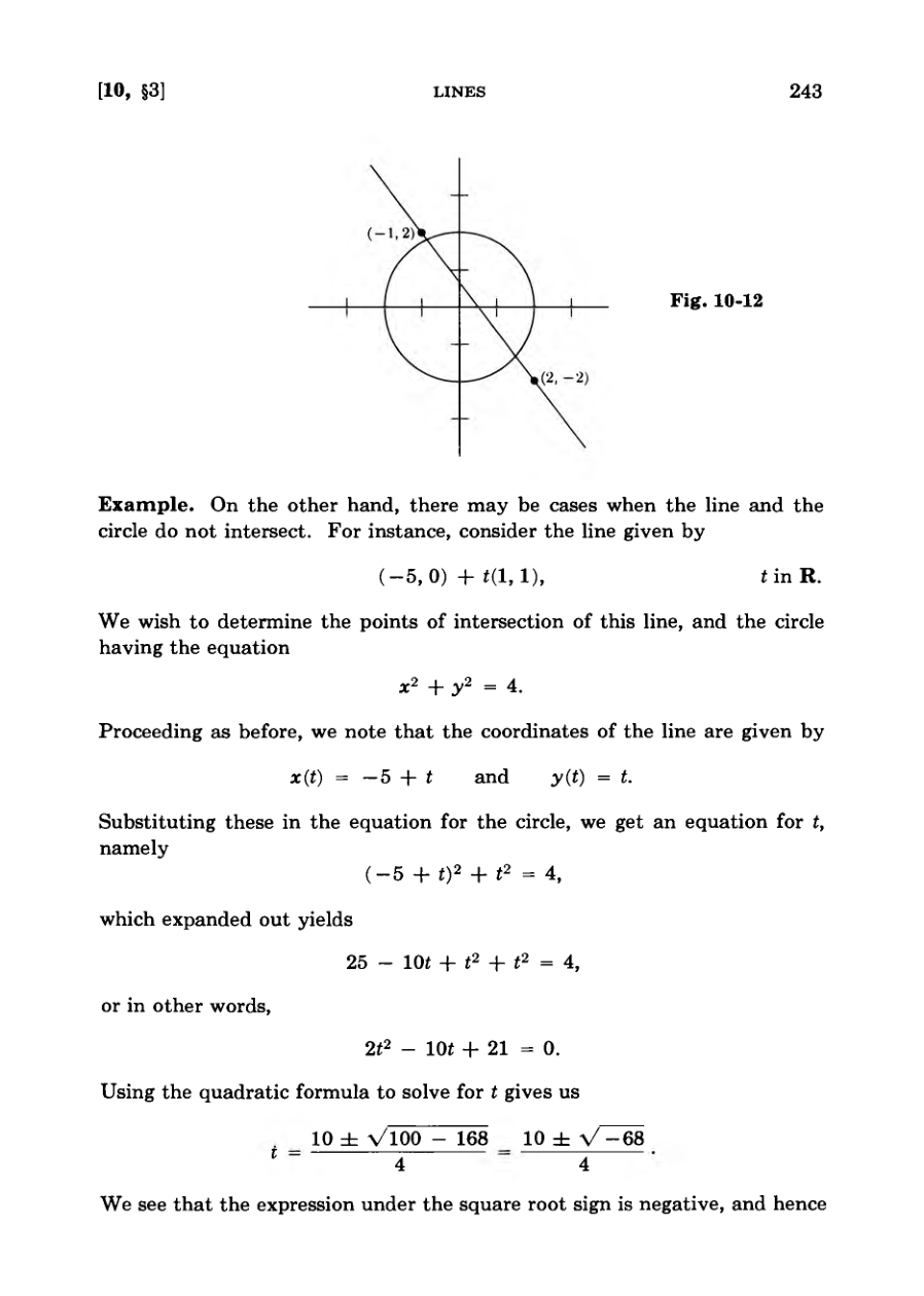
The intersection of a line and a circle can be determined by substituting the parametric equations of the line into the circle's equation.
Solving the resulting quadratic equation yields the parameter values for the points of intersection.
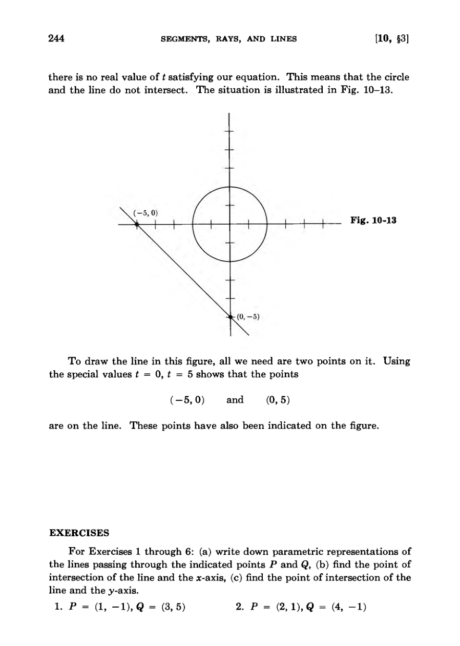
A negative discriminant in the quadratic equation indicates that the line and the circle do not intersect.
Practical exercises apply these algebraic methods to find intersections with axes and determine potential collision points for moving objects.
We see that the expression under the square root sign is negative, and hence there is no real value of t satisfying our equation.
DiagramDiagram
Ordinary Equation of a Line
Exercises require calculating intersections of given lines with each other and various circles.
Propositions include proving when two vectors are parallel and demonstrating that non-parallel lines intersect at a single point.
The text introduces the concept of converting parametric line representations into ordinary equations by eliminating the parameter t.
An algebraic example demonstrates finding the Cartesian equation 7x + 2y = 31 from a parameterized line.
Subsequent exercises ask readers to find ordinary equations for lines given in parametric form.
So far we have described a line in terms of a parameter t. We can eliminate this parameter t and get another type of equation for the line.
Diagram
Understanding Radian Measure
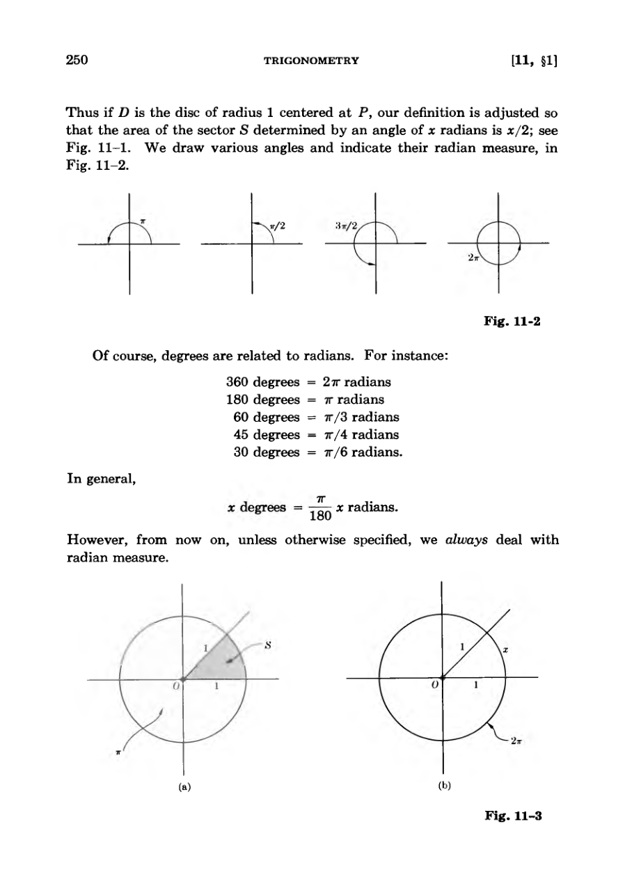
Degrees are described as a less natural measurement of angles compared to radians.
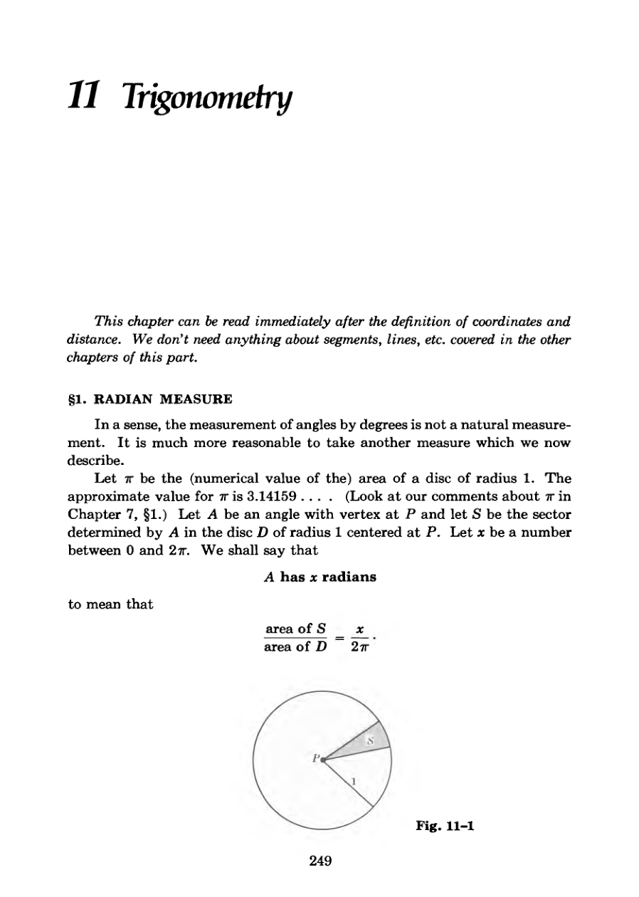
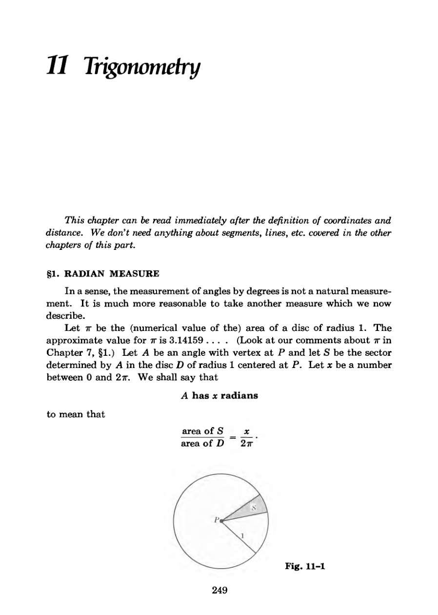
Radian measure is defined using the ratio of the area of a circular sector to the total area of a disc of radius one.
Radian measure also corresponds directly to the arc length on a unit circle.
Historical choices led to the frequent appearance of the constant two pi, which the author notes is slightly inconvenient.
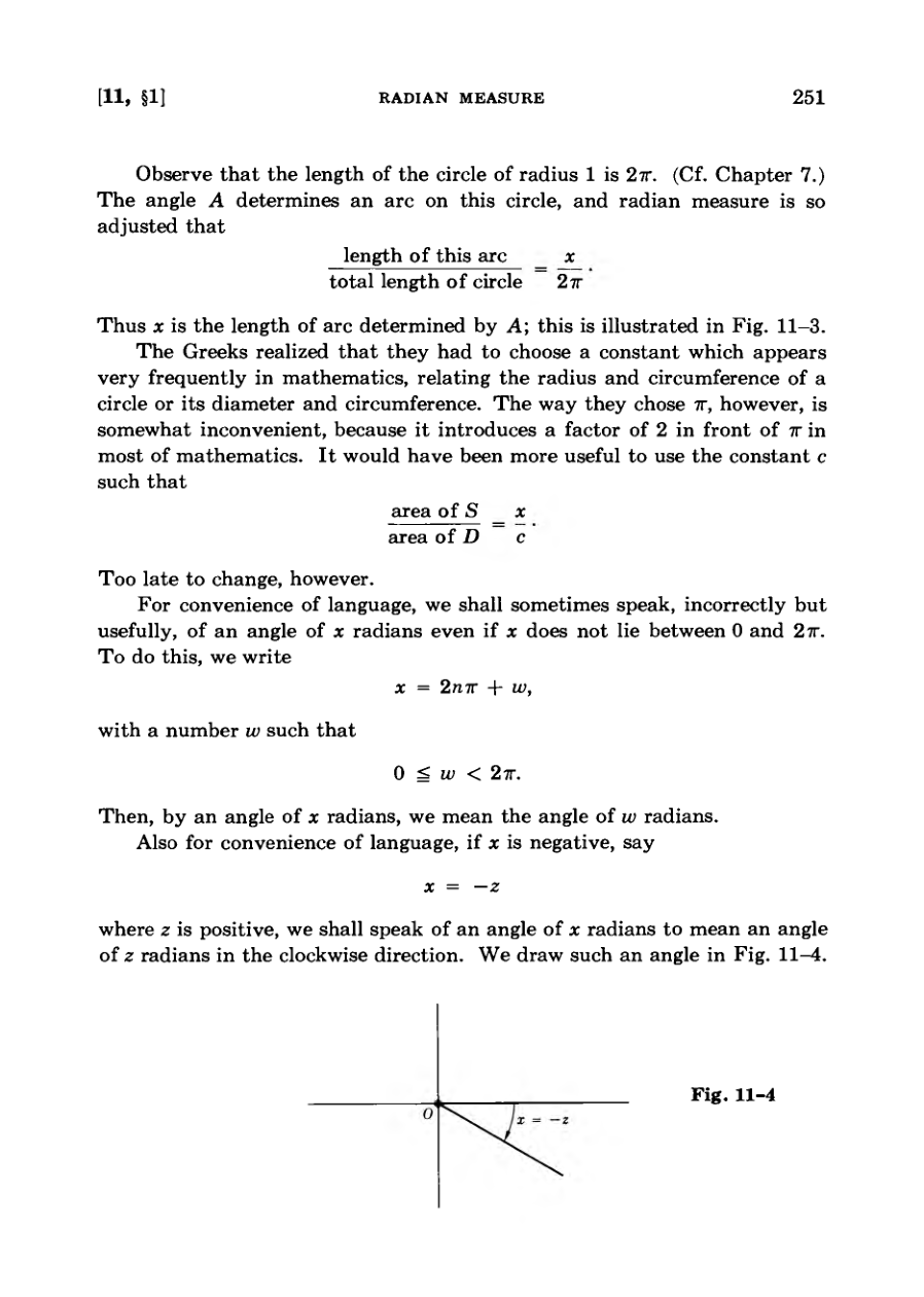
Negative angles and angles greater than two pi are accommodated by extending the definition through modular arithmetic.
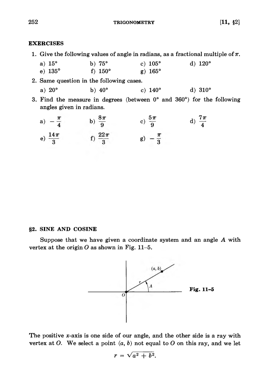
Sine and cosine are formally defined using the coordinates of a point on the ray of an angle and the distance from the origin.
Too late to change, however.
DiagramDiagramDiagramDiagramFigure
Defining Sine and Cosine
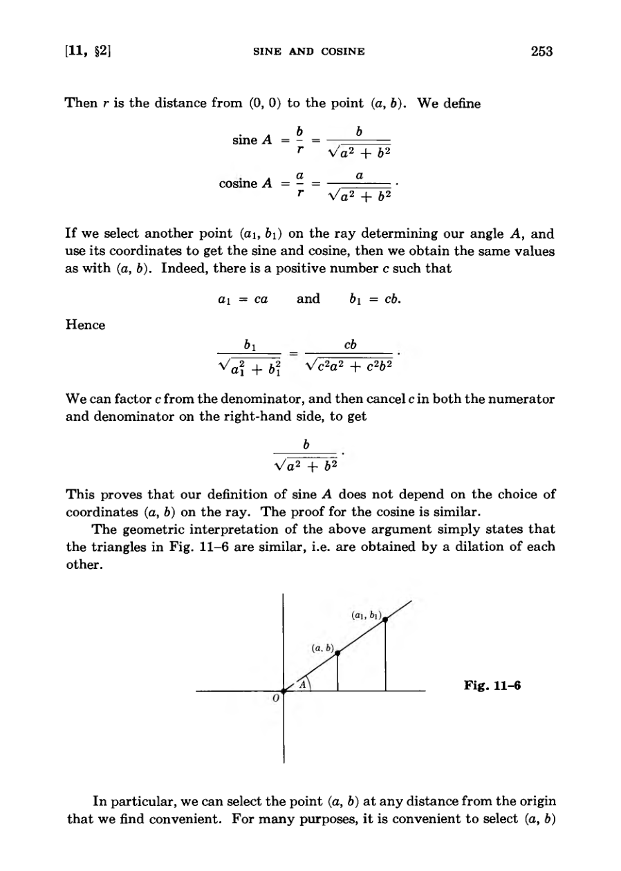
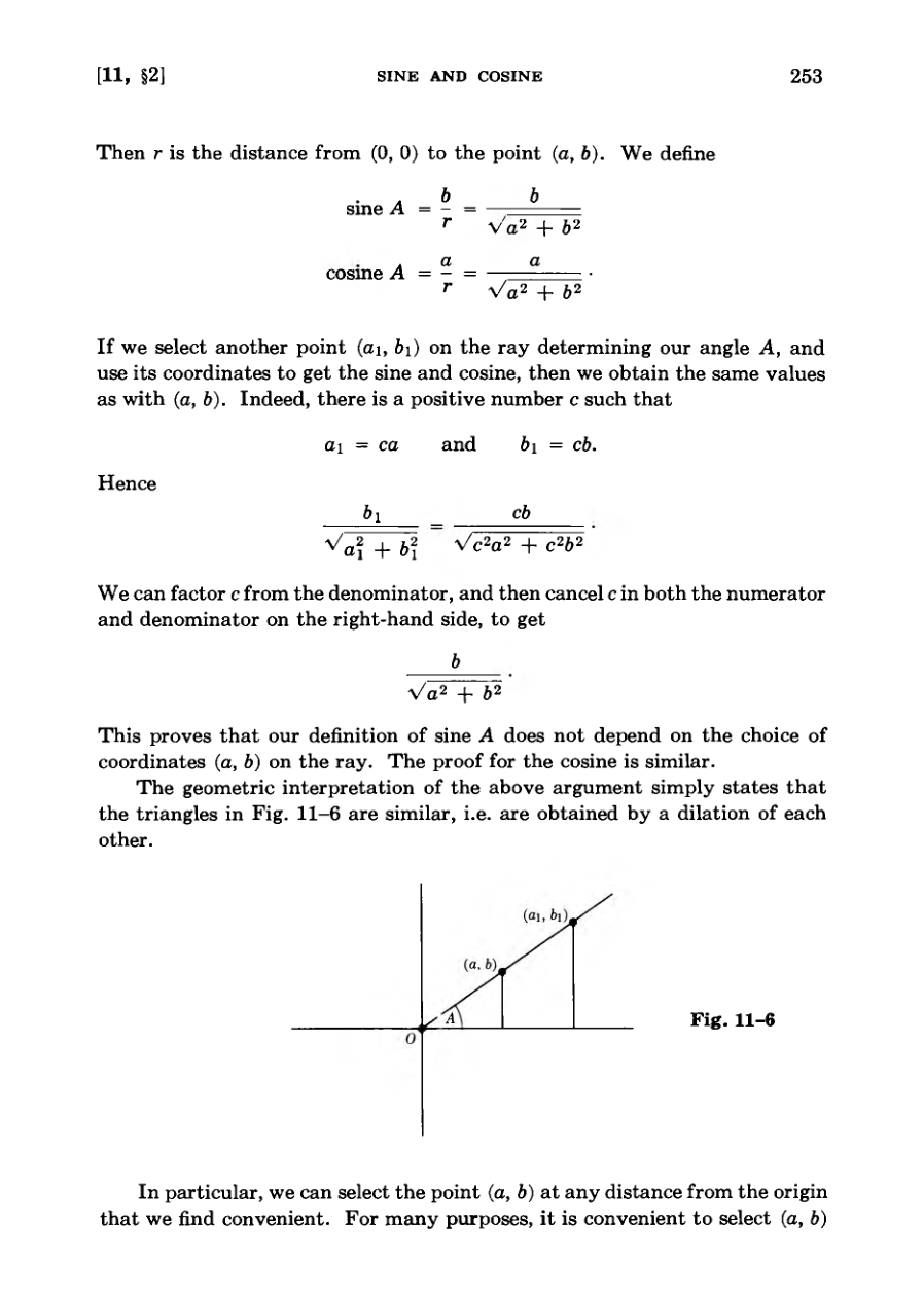
The definition of sine and cosine is independent of the choice of coordinates on a ray and relates directly to similar triangles.
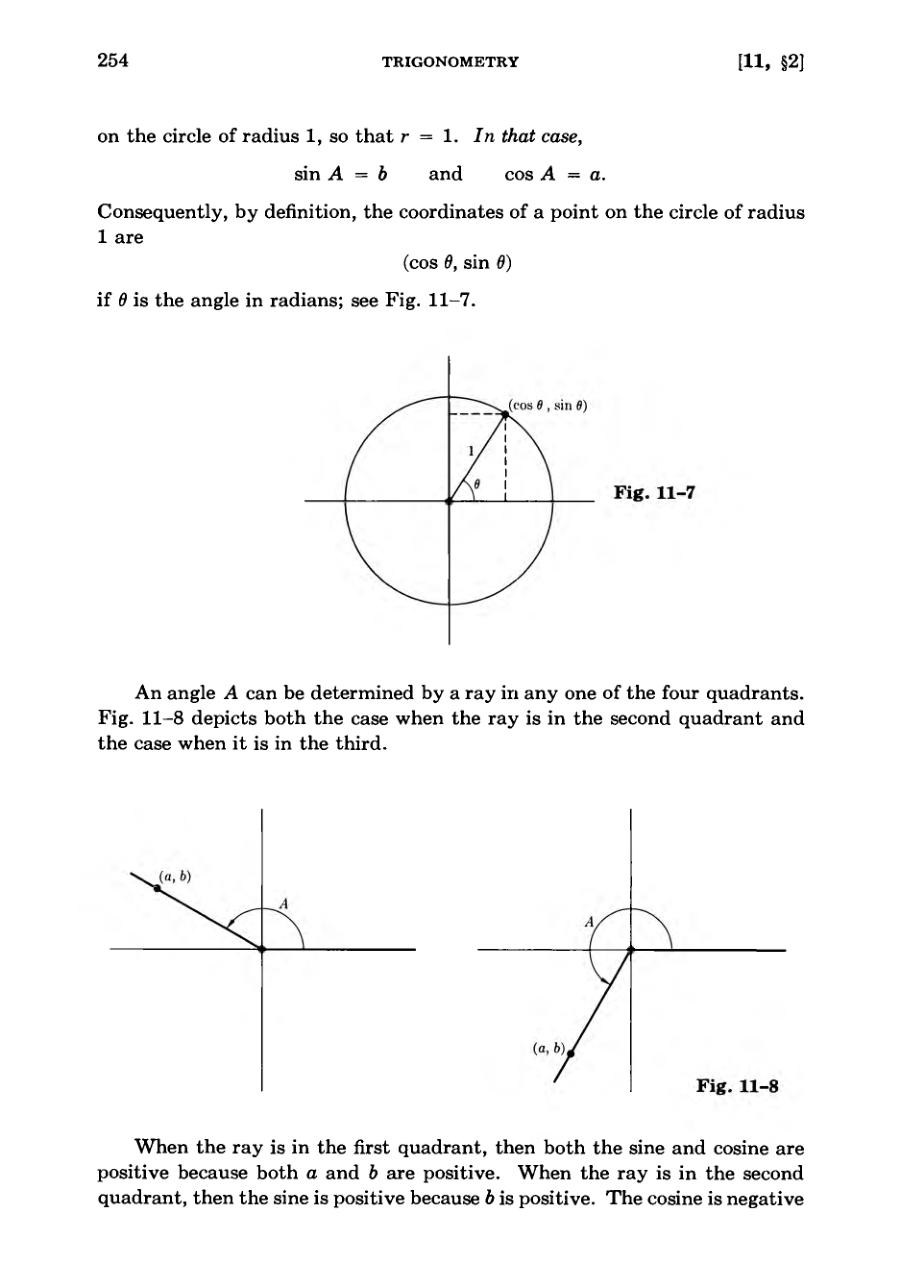
Using a unit circle of radius 1, the coordinates of any point become simply the cosine and sine of the corresponding angle.
The signs of the sine and cosine functions vary across the four quadrants based on the positive or negative values of the coordinates.
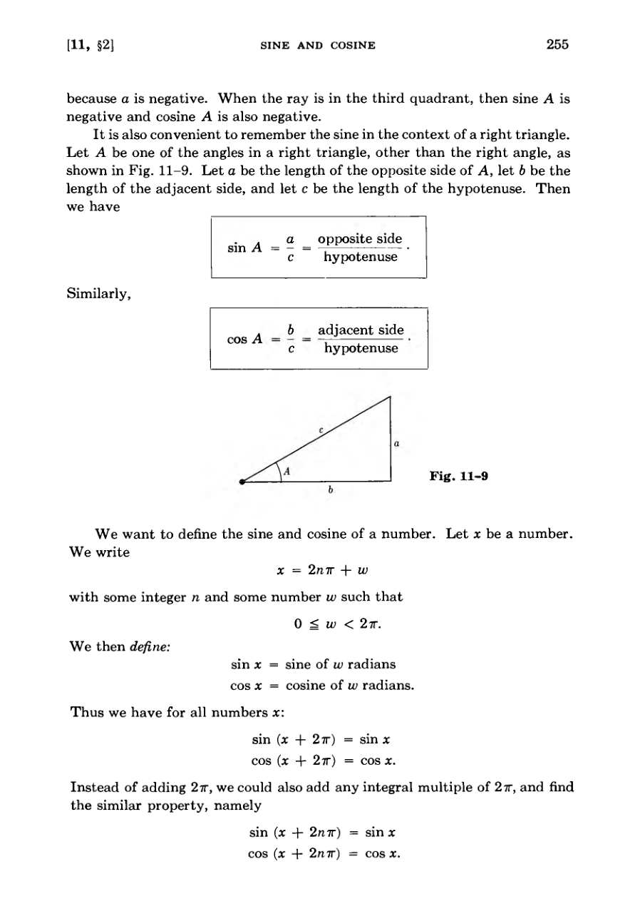
Sine and cosine can also be interpreted using right triangles as the ratios of the opposite or adjacent sides to the hypotenuse.
Extending these concepts to all numbers involves periodic functions that repeat every two pi radians.
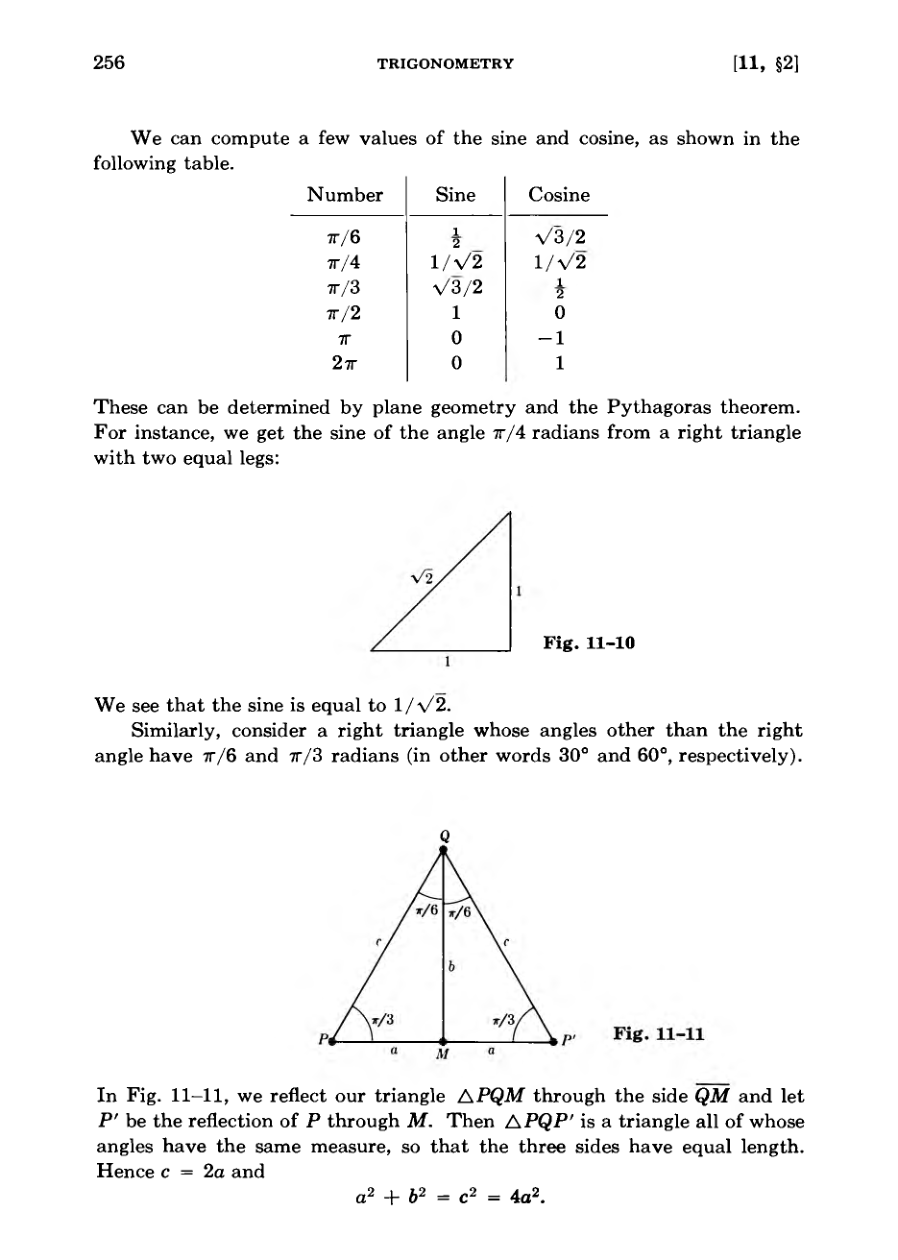
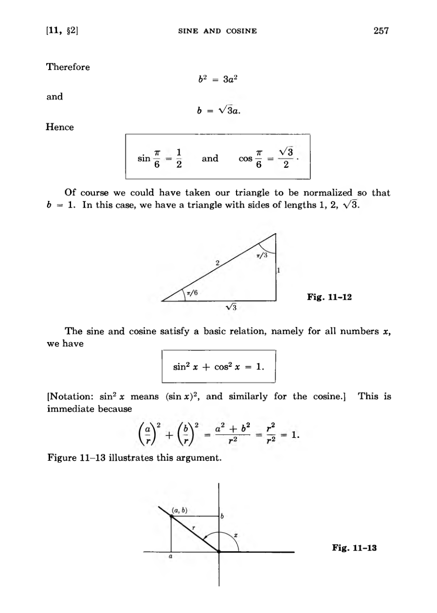
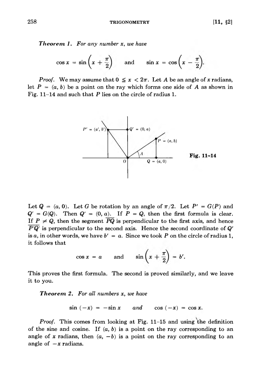
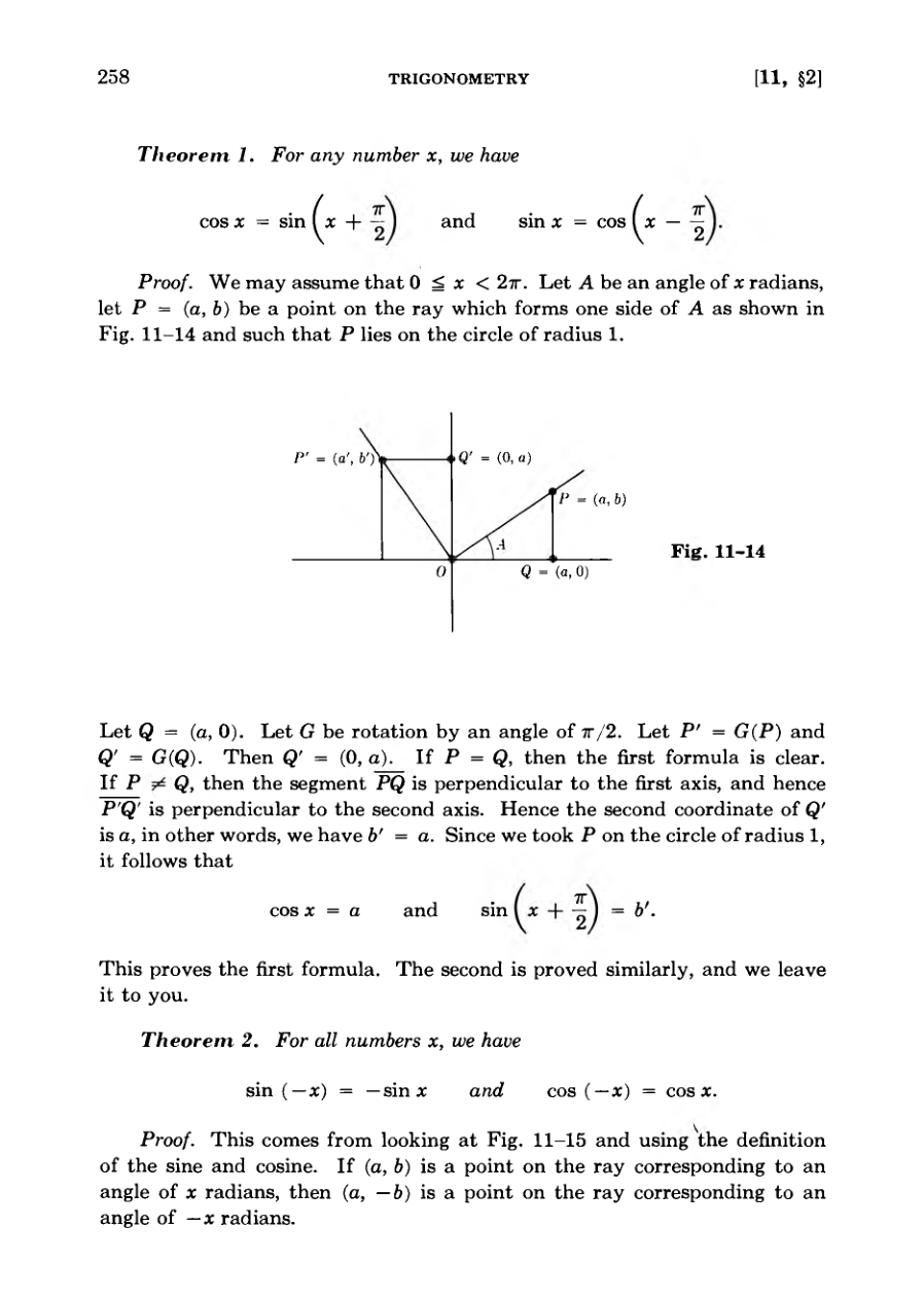
Basic values for sine and cosine can be computed using plane geometry, the Pythagorean theorem, and special right triangles.
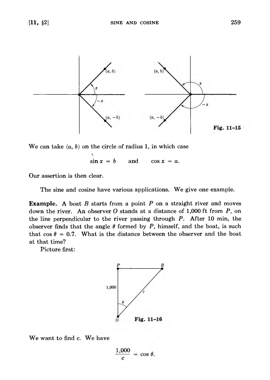
Consequently, by definition, the coordinates of a point on the circle of radius 1 are (cos 0, sin 0) if 0 is the angle in radians.
FigureDiagramDiagramDiagramDiagramDiagram
Trigonometry and Polar Coordinates
Proofs for trigonometric identities involving rotations and angle symmetries such as negative angles.
Practical applications of trigonometry to measure distances using small-sized instruments.
Introduction of polar coordinates as an alternative way to describe points in a plane using distance and angle.
Conversion formulas relating Cartesian coordinates to polar coordinates through sine and cosine.
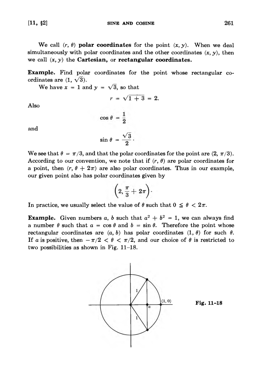
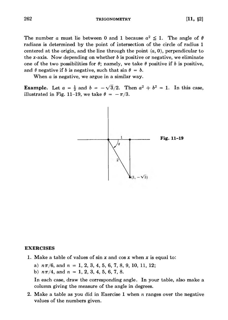
Examples illustrating how to find polar coordinates from rectangular coordinates and addressing multiple angle representations.
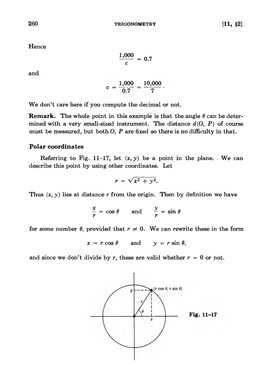
The whole point in this example is that the angle theta can be determined with a very small-sized instrument.
DiagramDiagramDiagramDiagram
Trigonometric Exercises and Graphs
The text explains how to determine angles and trigonometric values using a unit circle based on coordinates.
A comprehensive set of exercises is provided covering sine and cosine values for various multiples of pi.
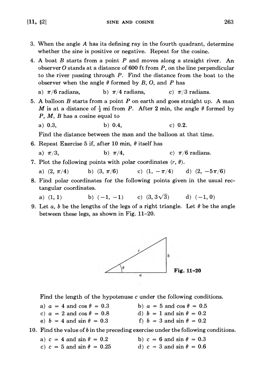
Practical word problems apply trigonometric concepts to real-world scenarios involving boats, balloons, and triangles.
Exercises also include plotting points and converting between polar and rectangular coordinates.
The final section introduces the study of the graphs of trigonometric functions starting with the sine function.
A boat B starts from a point P and moves along a straight river.
DiagramDiagram
Behavior and Graphs of Trigonometric Functions
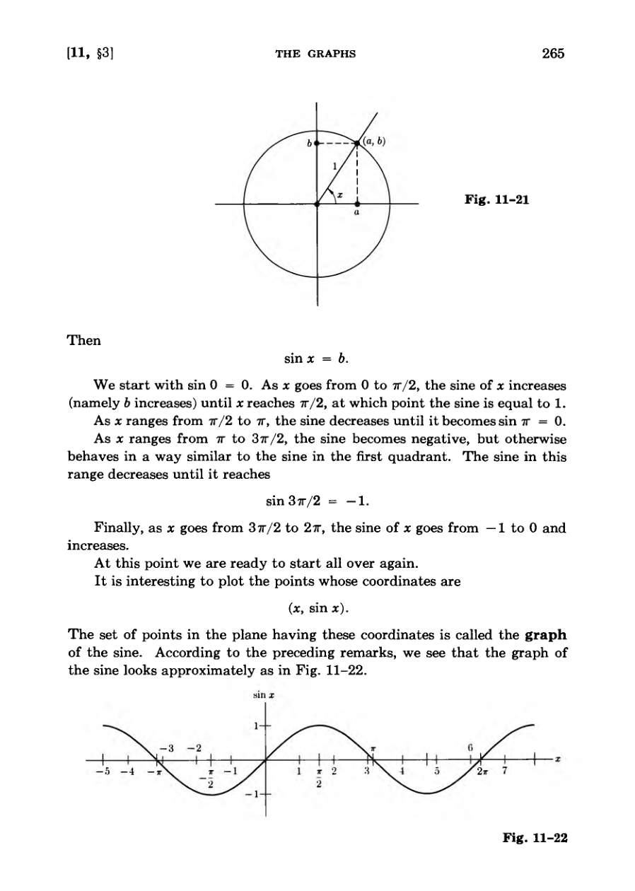
The sine function oscillates between 1 and -1 across four quadrants, repeating its cycle every 2pi units.
Plotting the points (x, sin x) creates the visual graph of the sine wave.
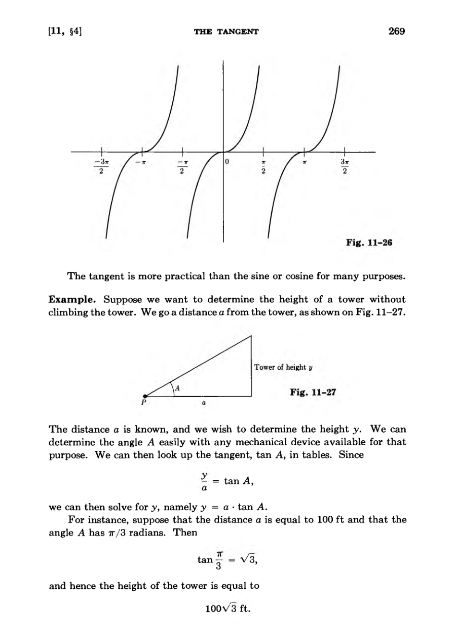
The tangent function is defined as the quotient of sine and cosine, and is undefined where the cosine equals zero.
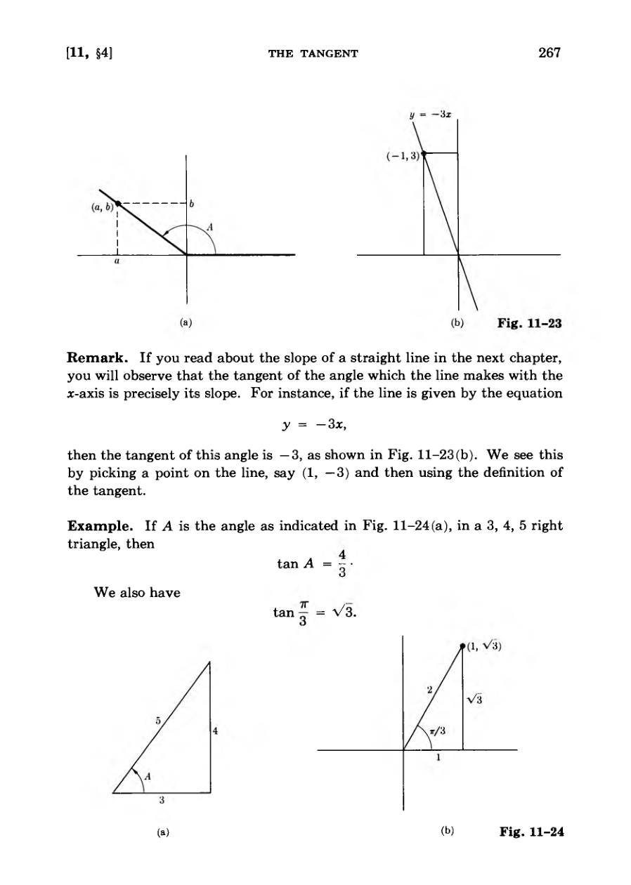
The tangent of the angle a line makes with the x-axis corresponds precisely to the slope of that line.
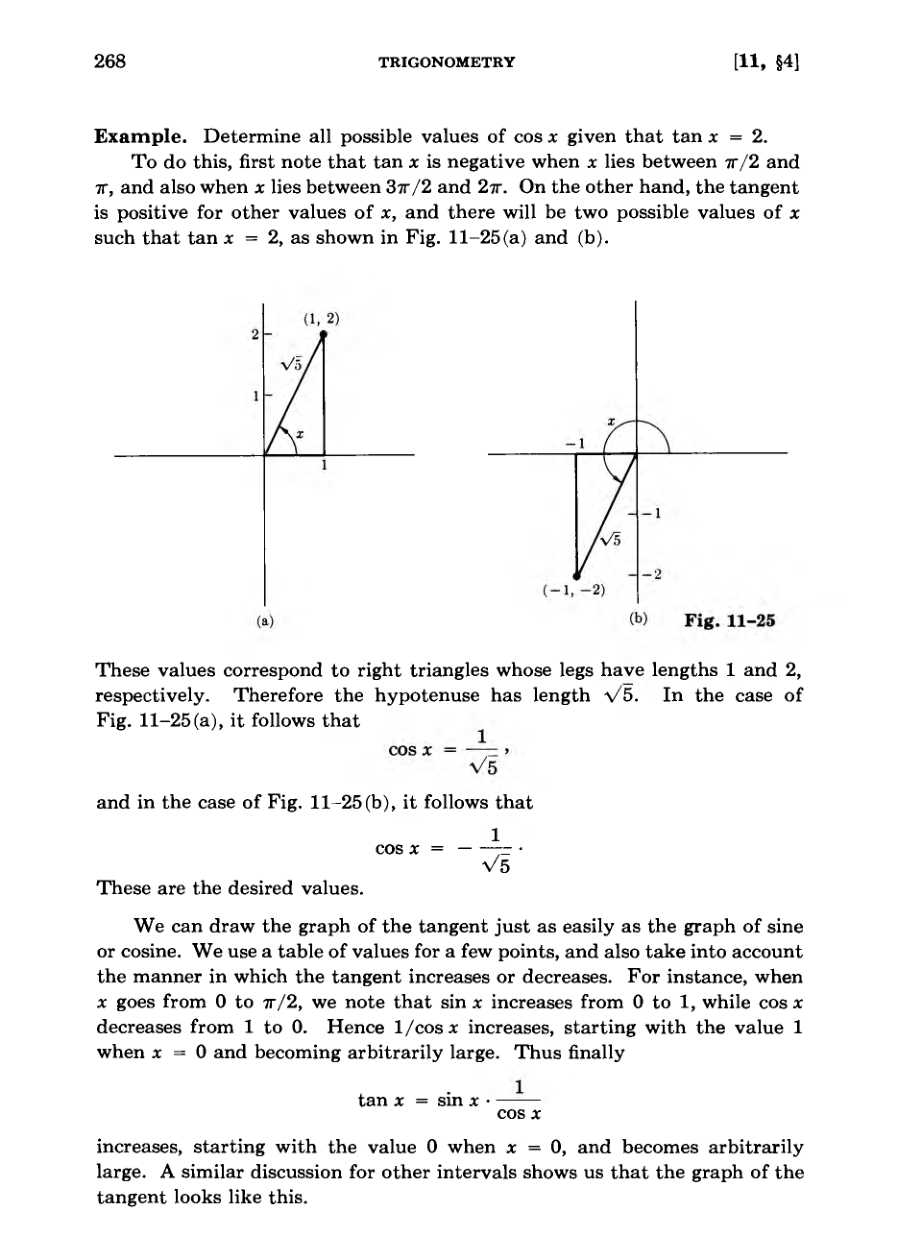
As x approaches pi/2, the tangent function increases from zero and becomes arbitrarily large.
If you read about the slope of a straight line in the next chapter, you will observe that the tangent of the angle which the line makes with the jc-axis is precisely its slope.
FigureDiagramDiagramFigure
Trigonometric Applications and Formulas
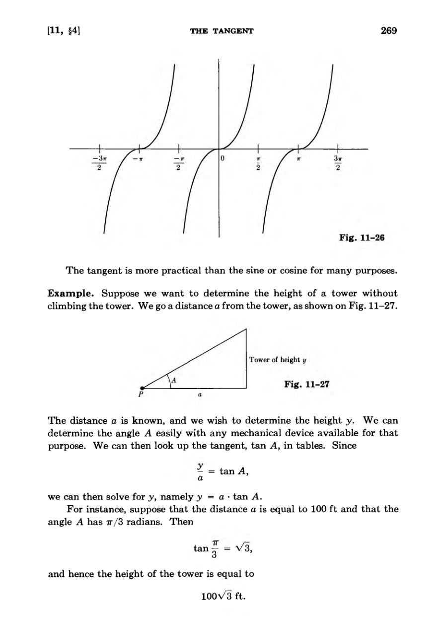
Trigonometry allows for indirect measurement of large objects like towers using known distances and angles.
The tangent function relates the opposite and adjacent sides of a right triangle to solve for unknown heights.
Exercises test understanding of trigonometric functions including cotangent, secant, and cosecant graphs.
Real-world word problems apply trigonometric ratios to buildings, rising balloons, and moving boats.
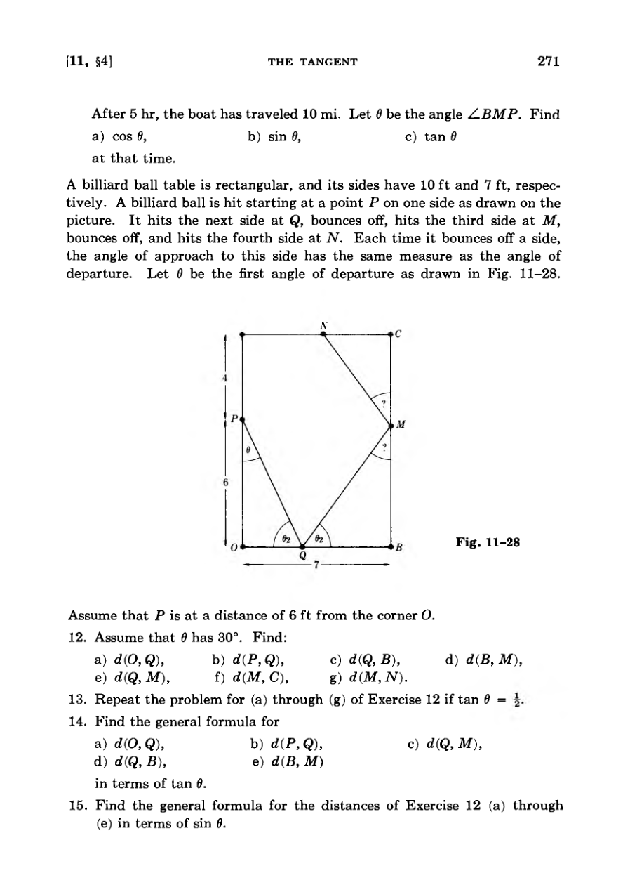
Geometric scenarios like billiard ball trajectories reinforce the practical application of angle measurements.
The section introduces foundational addition formulas for sine and cosine for any given angles.
Suppose we want to determine the height of a tower without climbing the tower.
FigureDiagramDiagram
Trigonometric Addition Formulas
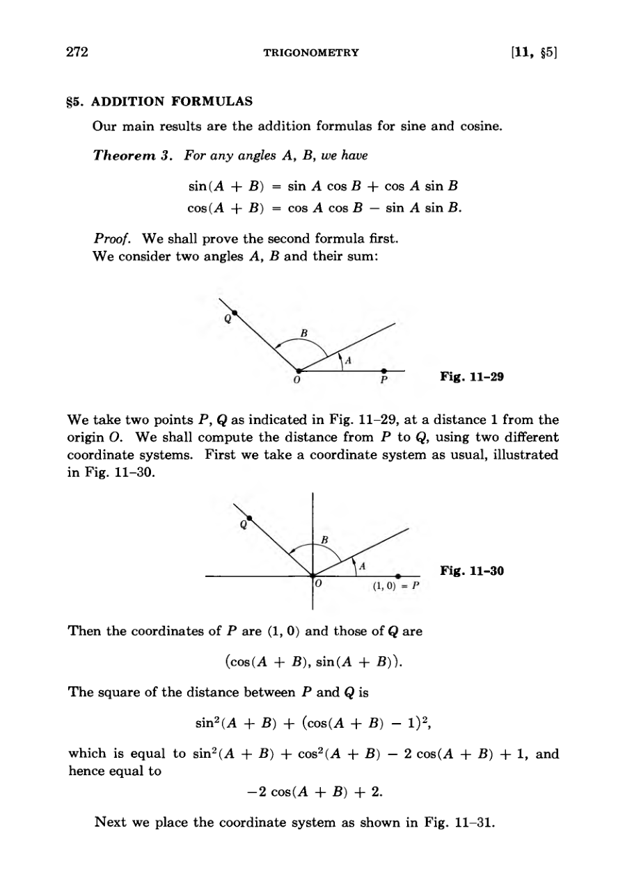
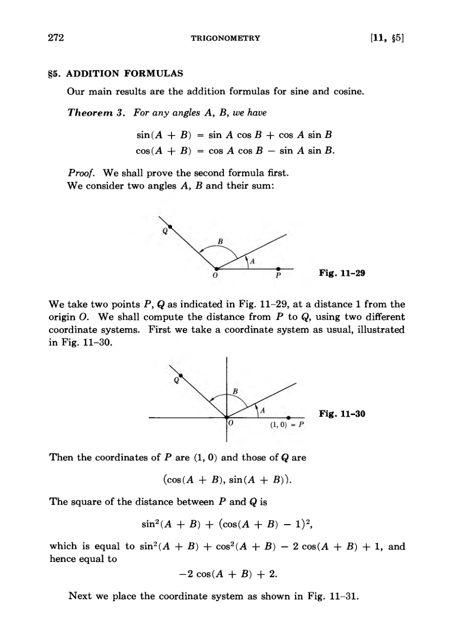
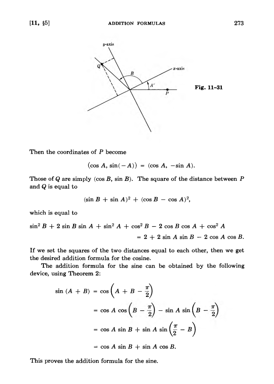
Distances between points on the unit circle are equated using two coordinate systems to derive the cosine addition formula.
The sine addition formula is subsequently proven by applying previously established identities to the derived cosine formula.
Corollaries provide subtraction formulas and fundamental identities like Pythagorean relations and negative angle rules.
Memorizing a select few core formulas allows for the efficient derivation of all other trigonometric identities.
Double-angle and half-angle formulas are demonstrated through practical examples involving specific angle measurements.
Read these out loud and get an aural memory of them.
DiagramDiagram
Trigonometric Identities and Rotations
The text presents various trigonometric exercises involving double-angle and half-angle formulas.
Practical applications include calculating maximum projectile distances for thrown balls and water streams using trigonometric identities.
The chapter transitions into investigating geometric rotations of points using coordinate systems and polar coordinates.
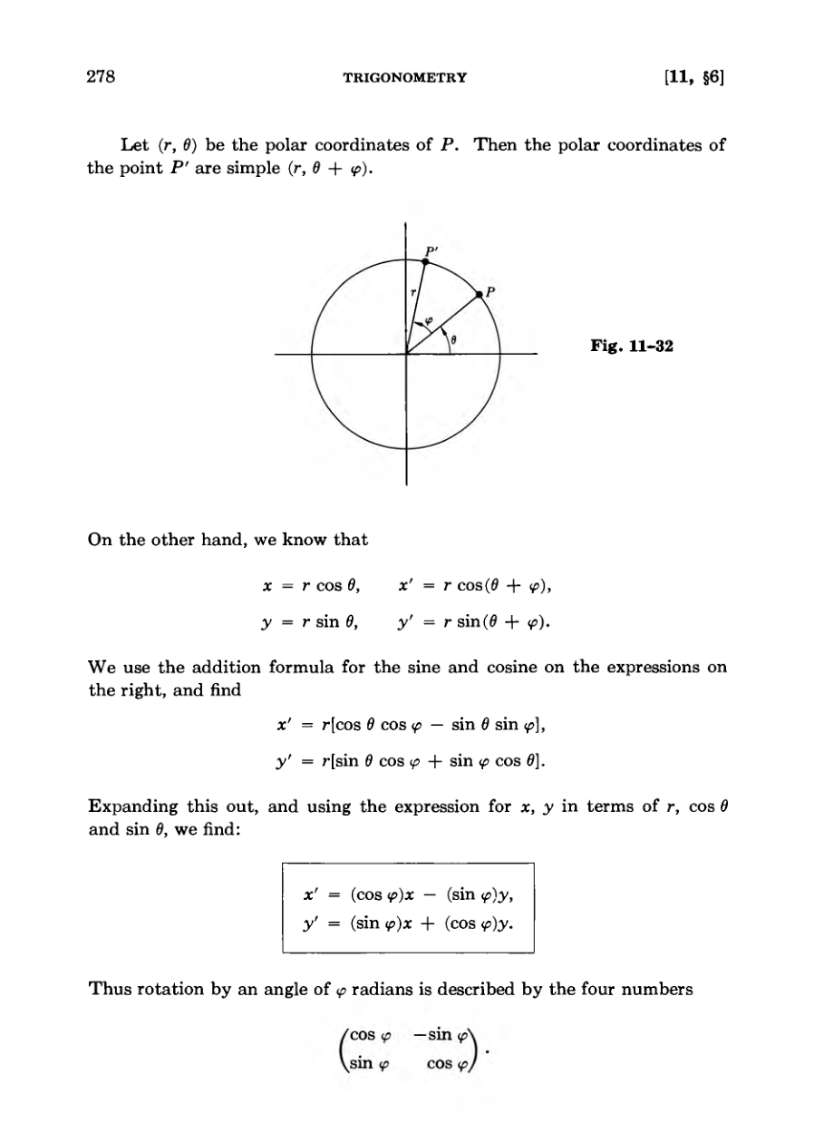
Addition formulas for sine and cosine are used to derive the new coordinates of a rotated point.
The resulting transformation equations for rotation naturally introduce the concept of a 2 by 2 matrix.
An array of numbers like has a technical name: It is called a matrix (in fact a 2 X 2 matrix).
Diagram
Matrix Multiplication and Analytic Geometry
Matrix multiplication defines linear transformations like rotations and dilations using 2 by 2 matrices.
Exercises prompt the calculation of coordinates and matrices for various rotation angles and dilations.
The text introduces analytic geometry by defining the graph of an equation F of x and y equals a constant c.
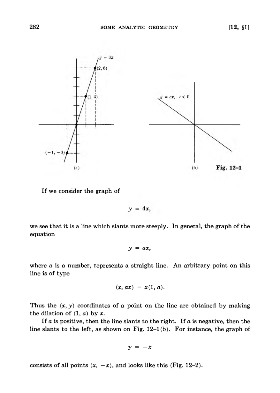
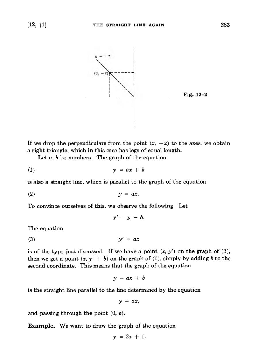
The simplest linear equation y equals ax represents a straight line through the origin whose slope depends on a.
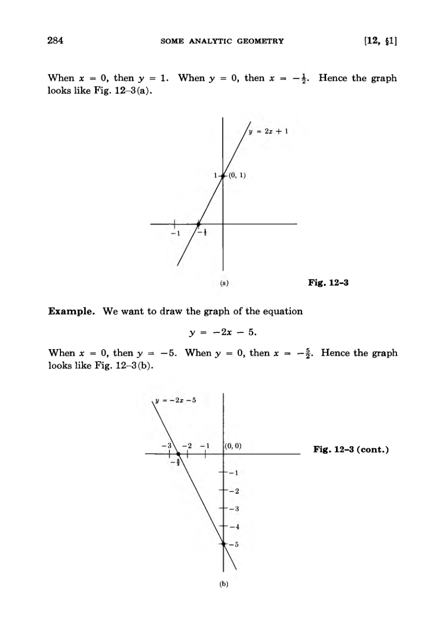
Adding a constant b to y equals ax shifts the line vertically, producing a parallel line that intersects the y axis at b.
This is something like a multiplication.
DiagramDiagramFigure
Understanding Line Slopes
The slope of a line determines its slant and can be identified directly from its equation.
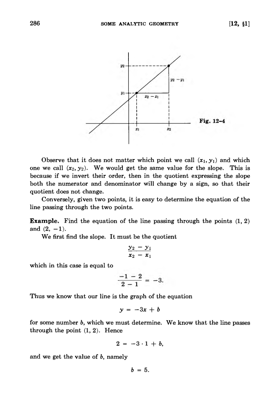
The slope formula calculates the ratio of the vertical change to the horizontal change between two distinct points.
Swapping the order of the two points does not change the calculated slope value.
The equation of a line can be determined using either two distinct points or a single point and the slope.
Vertical lines cannot be expressed in standard slope-intercept form and require a constant x-coordinate equation.
Line equations can be combined with circle equations to algebraically find their points of intersection.
Observe that it does not matter which point we call (x1,y1) and which one we call (x2,y2).
Diagram
Lines and Circles Intersection
Algebraic methods can determine the points of intersection between a line and a circle by substituting equations.
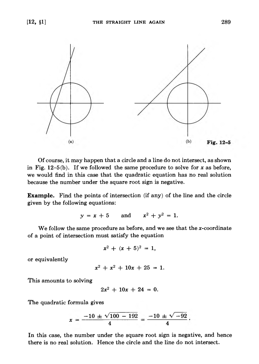
A negative value under the square root in the resulting quadratic equation indicates that the line and circle do not intersect.
Examples demonstrate both intersecting cases with real coordinates and non-intersecting cases yielding no real solutions.
A comprehensive set of exercises provides practice in sketching lines, finding intersection points, and determining line equations.
Special problems explore parallel lines, parametric forms, and various geometric configurations involving circles and lines.
If we followed the same procedure to solve for x as before, we would find in this case that the quadratic equation has no real solution because the number under the square root sign is negative.
Diagram
The Geometry of Parabolas
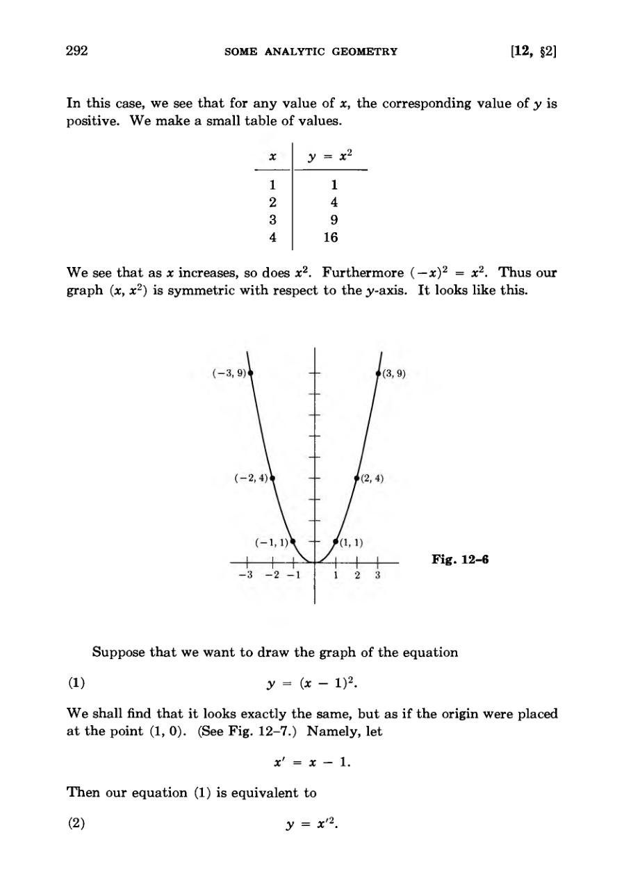
The basic graph of the equation y equals x squared is symmetric with respect to the y-axis and opens upward.
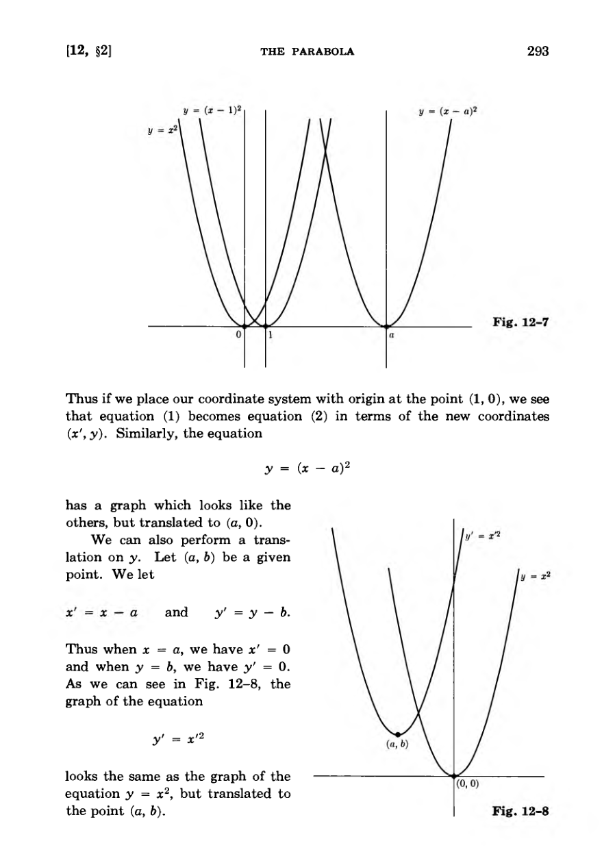
Substituting variables like x minus a allows us to translate the parabola horizontally to a new origin at (a, 0).
Performing translations on both x and y yields the general vertex form of a parabola shifted to the point (a, b).
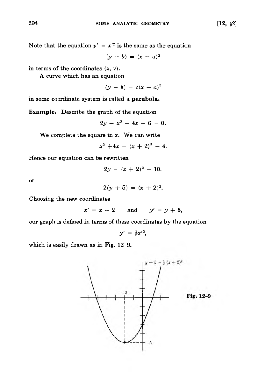
Completing the square helps rewrite quadratic equations into standard parabolic coordinate forms that are easy to sketch.
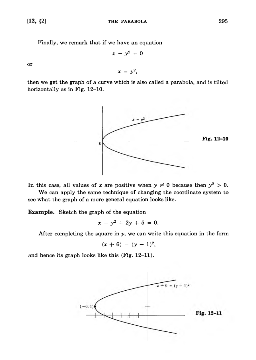
Parabolas also appear oriented horizontally when expressed in the form x equals y squared.
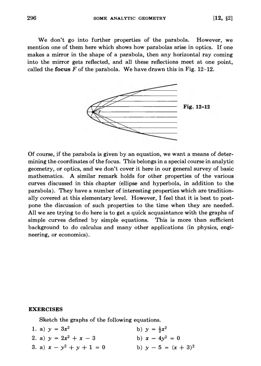
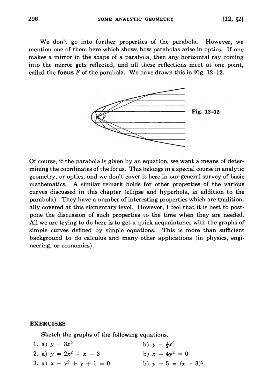
Beyond analytic geometry, parabolic mirrors possess the unique optical property of reflecting incoming horizontal rays to a single focal point.
If one makes a mirror in the shape of a parabola, then any horizontal ray coming into the mirror gets reflected, and all these reflections meet at one point, called the focus F of the parabola.
FigureFigureFigureFigureDiagram
Analytic Geometry of Ellipses
The text provides various quadratic equation graphing exercises involving parabolas and completing the square.
It introduces the concept of coordinate dilation, where multiplying coordinates by positive numbers stretches the plane.
A mixed dilation applied to the unit circle transforms it into a new geometric figure known as an ellipse.
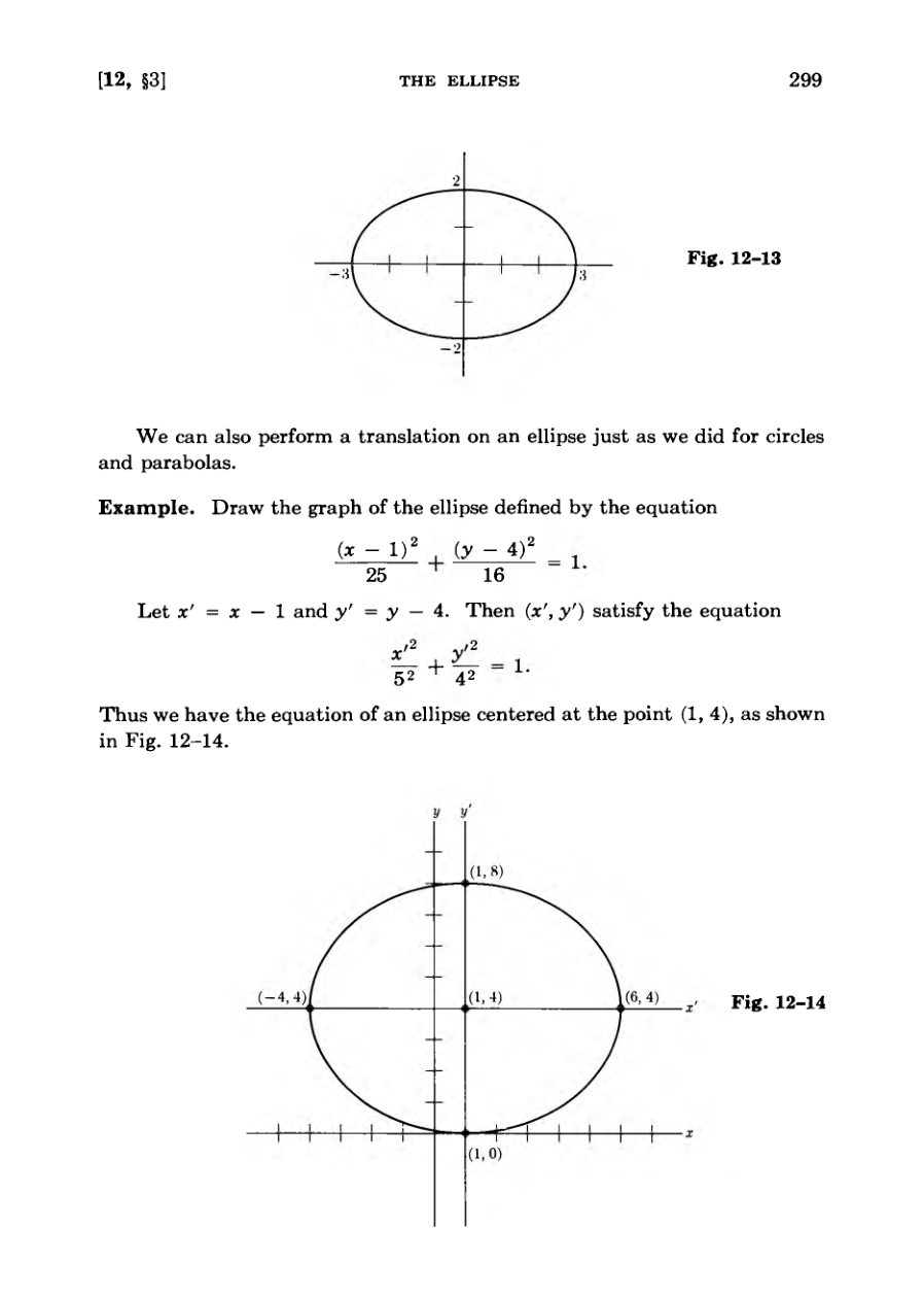
Ellipses can also undergo translations to shift their centers away from the origin in a coordinate system.
Exercises at the end require students to sketch various ellipses, find their centers and extremities, and calculate intersection points.
Hence the image of the circle defined by equation (1) is the set of points (u, v) satisfying equation (2).
DiagramFigure
Graphing the Hyperbola
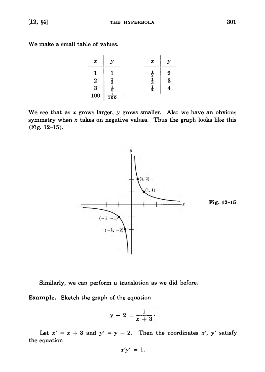
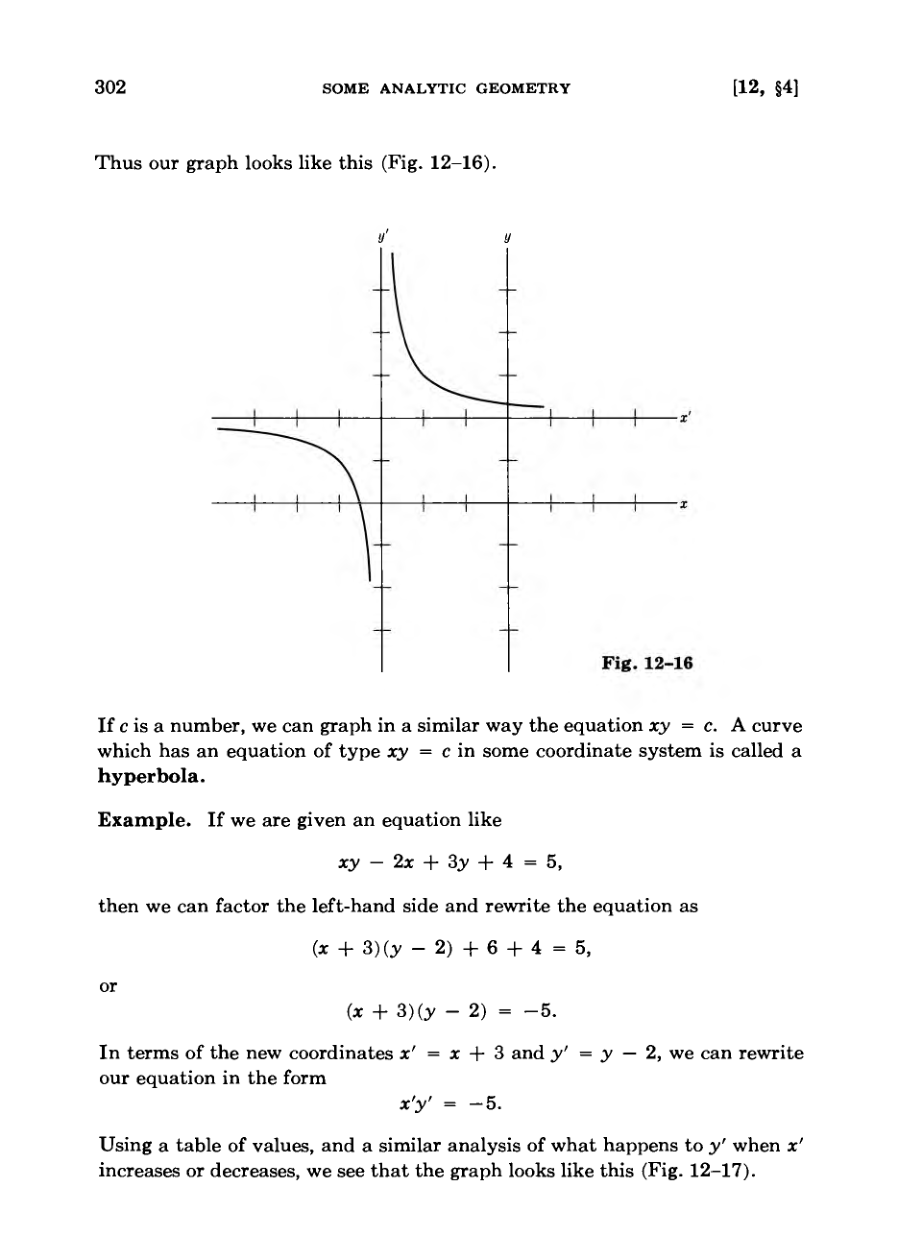
The basic equation xy = 1 forms a hyperbola where neither x nor y can equal zero.
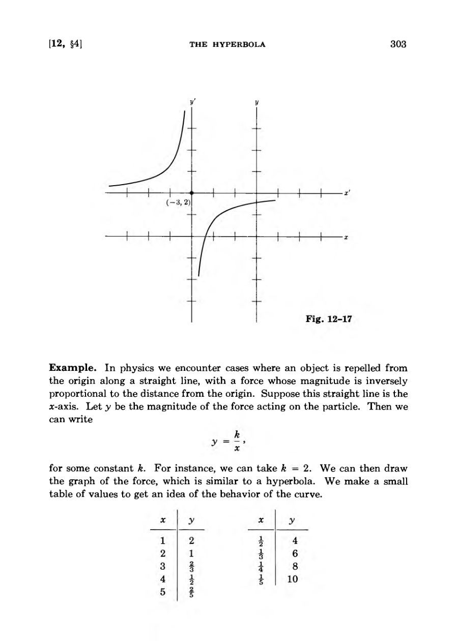
Translations allow complex equations like xy - 2x + 3y + 4 = 5 to be rewritten into standard hyperbola forms.
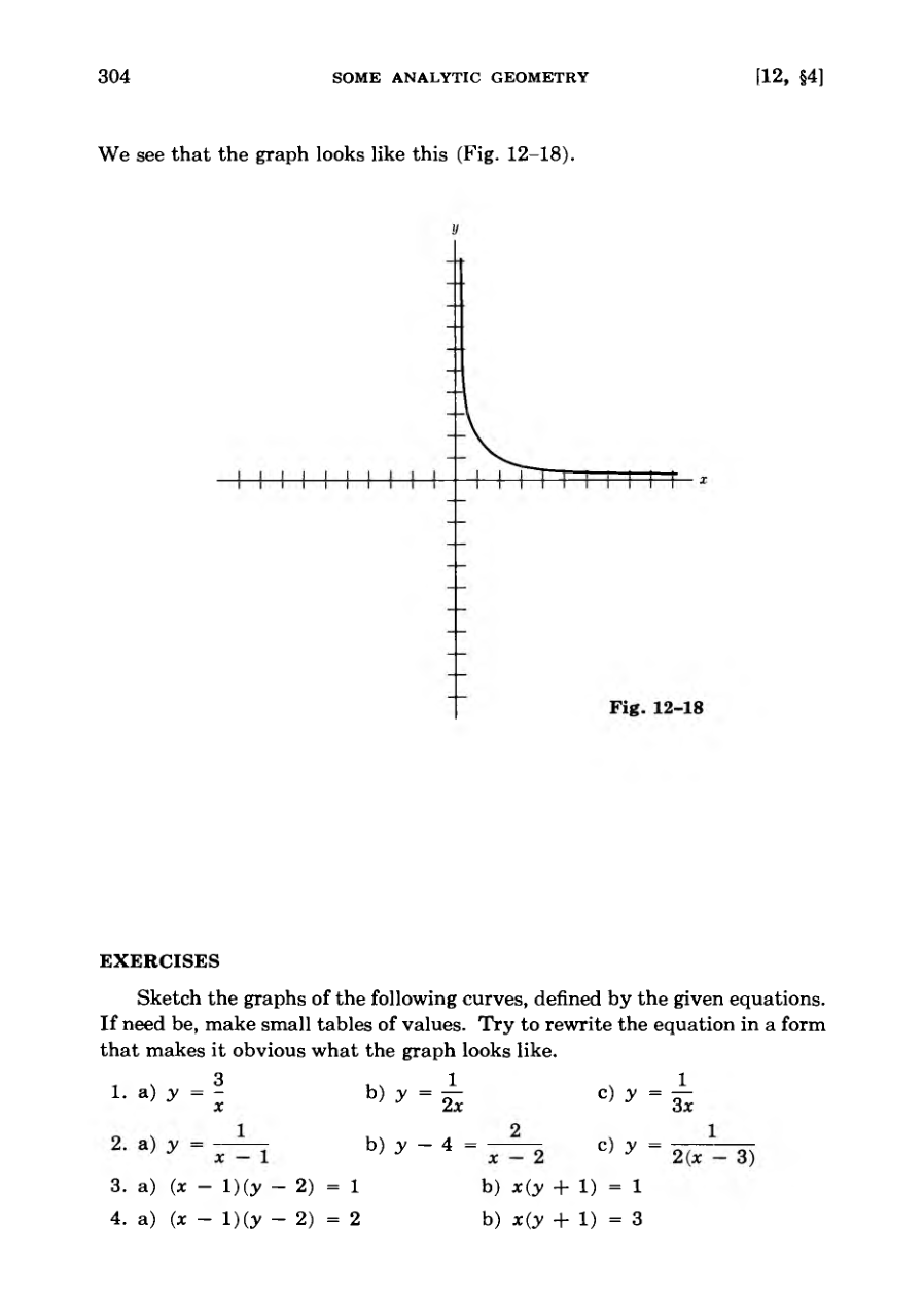
Hyperbolas naturally model physical phenomena, such as forces inversely proportional to distance.
Coordinate transformations using new variables simplify the sketching of shifted hyperbola curves.
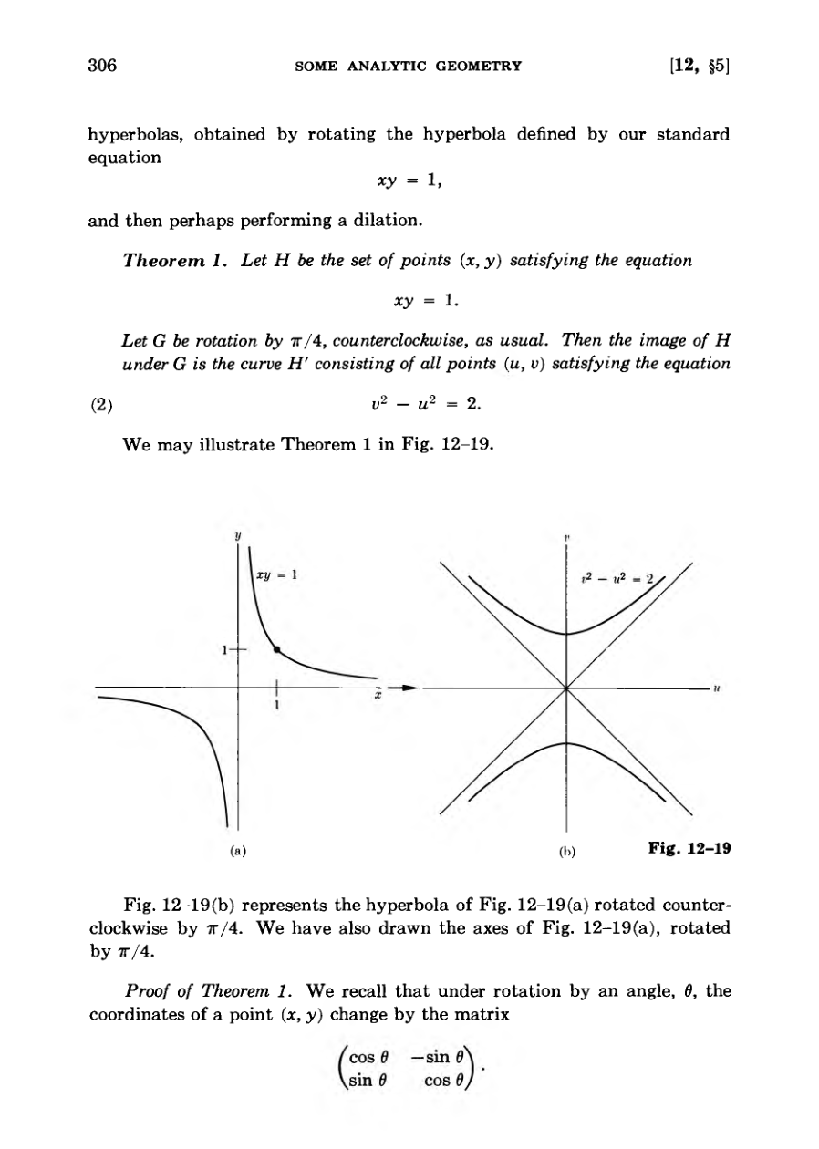
Rotations of standard hyperbolas produce alternative equations like y squared minus x squared equals c.
In physics we encounter cases where an object is repelled from the origin along a straight line, with a force whose magnitude is inversely proportional to the distance from the origin.
FigureFigureFigureFigureFigure
Rotation of Hyperbolas
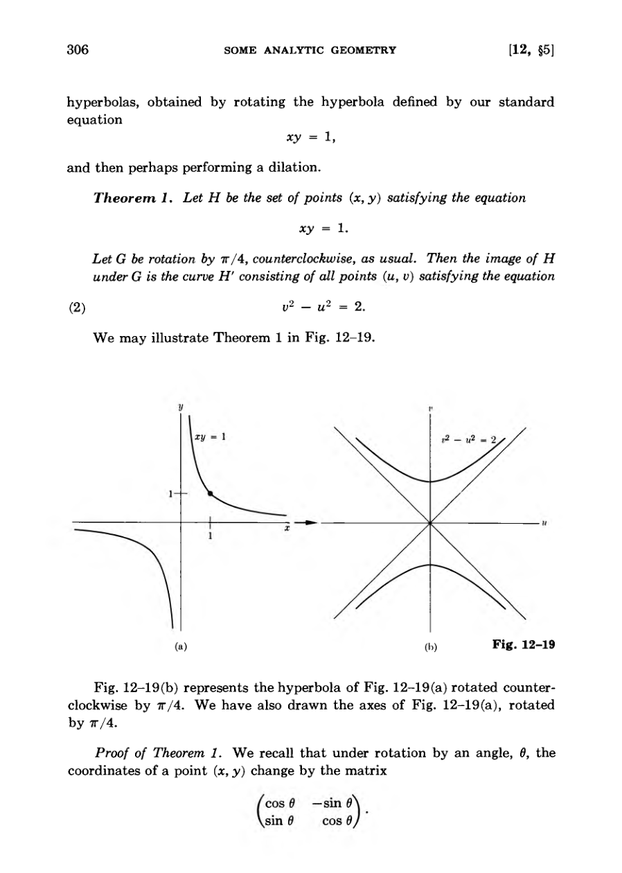
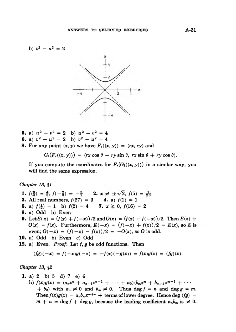
The text proves Theorem 1 by demonstrating that rotating the hyperbola defined by xy = 1 by an angle of pi/4 results in the equation v^2 - u^2 = 2.
The inverse proof confirms that any point satisfying the rotated equation can be mapped back to the original hyperbola by rotating through an angle of -pi/4.
Hyperbolas defined by xy = r^2 are shown to be dilations of the standard hyperbola by a factor of r.
The mathematical principle is established that a rotation commutes with a dilation, meaning dilating followed by rotation yields the same result as rotating followed by dilation.
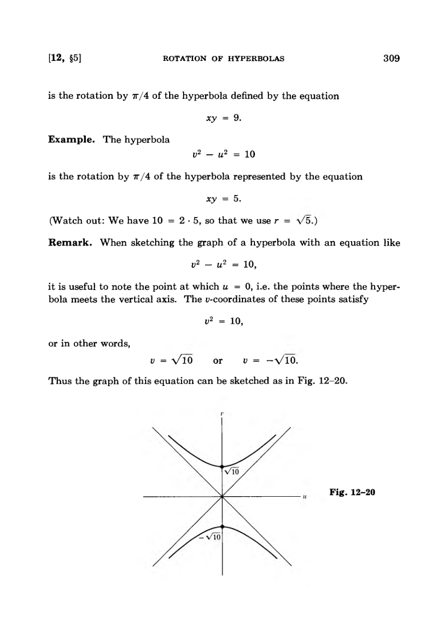
Practical examples illustrate how rotated hyperbola equations relate to their original coordinate forms and how to find their axis intersections for sketching.
Our intuition immediately tells us how to find (x, y ) : these coordinates are obtained by rotating (u, v) through an angle of — 7r/4.
FigureFigure
Hyperbolas and Functions
Exercises involve sketching various hyperbolas, finding their rotated images, and proving algebraic properties of geometric transformations.
Part Four introduces functions, defining them as associations between numbers where each input corresponds to a specific output value.
Functions can be represented by formulas like squares and sums, trigonometric rules, or constant values.
The definition of a function is extended to subsets of numbers, such as restricting square roots to non-negative numbers.
Functions can also be defined arbitrarily, such as assigning zero to rational numbers and one to irrational numbers.
The sum of two functions is defined by adding their values element-wise, inheriting standard algebraic properties like associativity and commutativity.
Let G be the function such that G(x) = 0 if x is a rational number, G(x) = 1 if x is not a rational number.
Algebraic Properties of Functions
Functions satisfy the same fundamental rules for addition and multiplication as ordinary numbers.
The zero function and constant unit function act as additive and multiplicative identities.
Multiplication of functions is commutative, associative, and distributive over addition.
Functions can be used to model real-world phenomena, such as historical population growth and subway fares.
Exercises explore function evaluations, even and odd symmetries, and the definition of polynomial functions.
In physical life, functions of numbers occur when we describe one quantity in terms of another.
Properties of Polynomial Roots
A polynomial of degree n must have a uniquely defined degree, meaning it cannot be represented by coefficient sets of varying lengths.
A number c is defined as a root of a polynomial f if substituting c into the polynomial yields zero.
Theorem 1 establishes that if c is a root of a polynomial f of degree n, then f can be factored as (x - c)g(x) where g is a polynomial of degree n minus one.
Theorem 2 proves that a polynomial with leading coefficient different from zero can have at most n distinct roots.
The process of successive factoring allows roots to be pulled out one by one until the remaining polynomial is reduced to a constant.
If the answer were YES, then it would be hopeless to define the degree, because in the example just written down, for instance, we would not know whether the degree is 5 or 6.
Uniqueness of Polynomial Coefficients
A polynomial has at most n roots based on previous theorems.
The corollary proves that the coefficients of a polynomial are uniquely determined.
The degree of a polynomial is defined by its highest non-zero coefficient power.
A polynomial evaluating to zero at a specific point is distinct from the zero polynomial.
Finding roots for polynomials of degree five or higher generally lacks a radical formula.
Excessive emphasis on factoring in elementary classes is discouraged in favor of systematic formulas.
It is very unusual that a polynomial can be factored with integral or rational roots, and I think much too much emphasis is placed on this kind of accident.
Polynomial Long Division
Polynomial factorization allows breaking down complex expressions into simpler roots and factors.
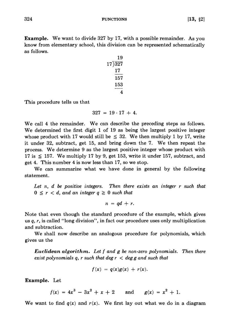
The division of polynomials parallels the traditional long division process used for positive integers.
Dividing integers yields a quotient and a remainder that is strictly less than the divisor.
The Euclidean algorithm for polynomials produces quotient and remainder polynomials based on their degrees.
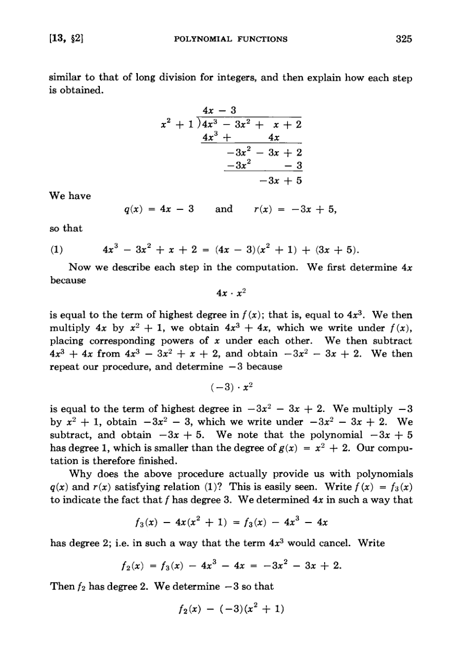
Each step in polynomial long division systematically eliminates the highest degree term through subtraction.
Note that even though the standard procedure of the example, which gives us q, r, is called “ long division” , in fact our procedure uses only multiplication and subtraction.
DiagramDiagram
Polynomial Euclidean Algorithm
The text demonstrates polynomial division and the Euclidean algorithm yielding a quotient and a remainder.
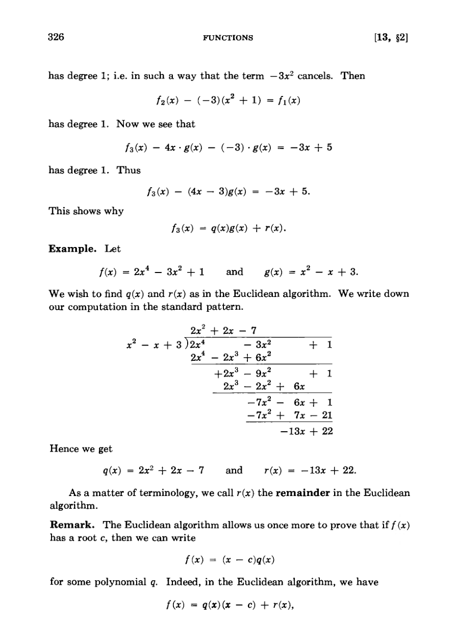
A concrete numerical example illustrates the step-by-step polynomial long division process.
The Euclidean algorithm provides a proof that if a polynomial has a root c, it can be factored by (x - c).
Exercises at the end test polynomial degrees, root finding, and the application of the Euclidean algorithm.
The section concludes by introducing rational functions as quotients of polynomials.
We do not prove the Euclidean algorithm. The proof would consist of carrying out the procedure of the example with general coefficients.
Figure
Rational Functions and Graphs
Combining rational functions over a common denominator results in another rational function, which can be expanded into polynomial form.
Exercises challenge the reader to practice expressing sums of various rational functions as quotients of polynomials.
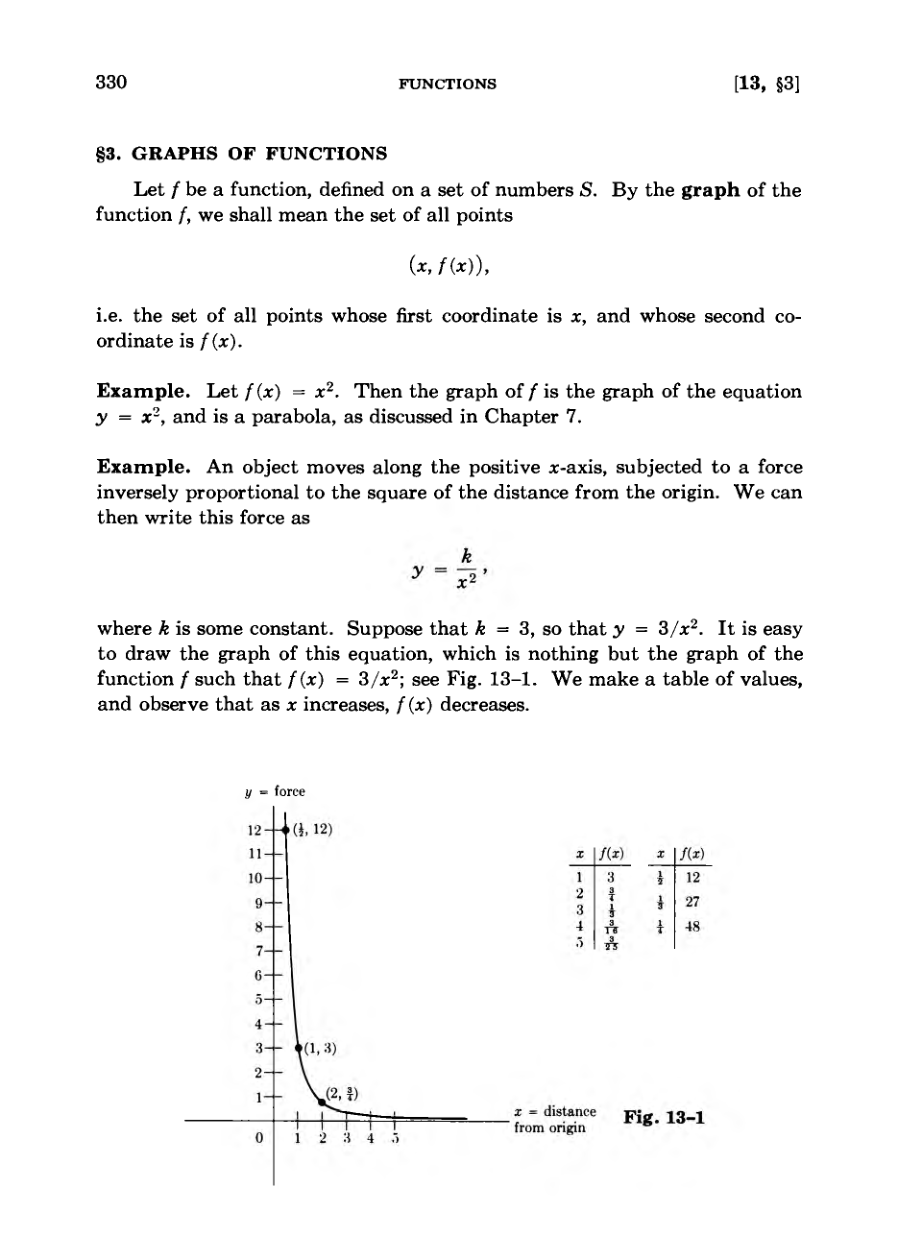
The graph of a function is formally defined as the set of all coordinate points (x, f(x)).
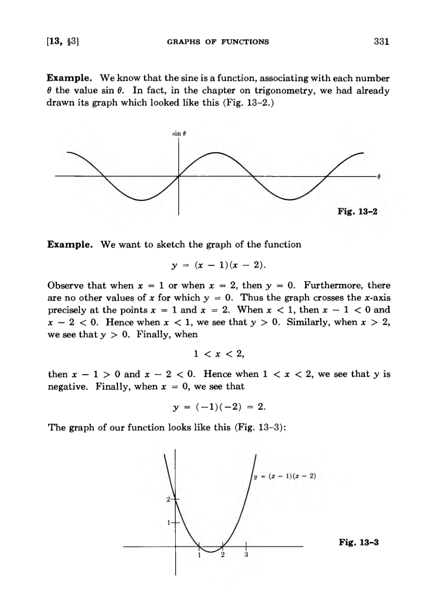
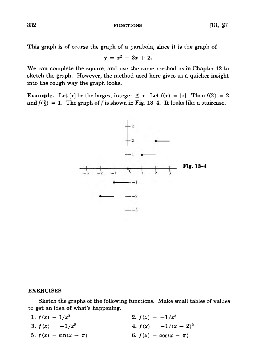
Examples of function graphs include parabolas, inverse square force relationships, trigonometric sine waves, and staircase-like integer step functions.
Analyzing where a function's value is zero, positive, or negative provides a quick and intuitive insight into the rough shape of its graph.
Let [x] be the largest integer ^ x.
GraphFigureFigure
The Exponential Function
The exponential function extends powers from integers and fractions to all real numbers using fundamental intuitive properties.
Basic algebraic rules govern the function, including rules for addition of exponents, power of a power, and products.
The exponential function is strictly increasing when the base is greater than one, yielding exclusively positive values.
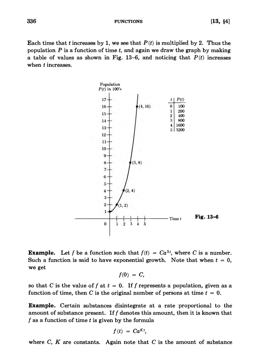
Practical phenomena such as population growth and radioactive disintegration can be effectively modeled using exponential functions.
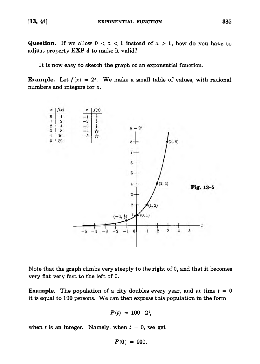
Graphs of exponential functions exhibit characteristic behavior, climbing steeply for positive inputs and flattening rapidly for negative inputs.
Certain substances disintegrate at a rate proportional to the amount of substance present.
FigureGraph
Exponential Growth and Logarithms
Textbook problems explore exponential decay and growth models involving radium, city populations, bacteria, and radioactive elements.
Logarithms are formally introduced as the inverse of exponential functions, defined when a > 1 such that if y equals a to the power of x, then x is the logarithm of y to the base a.
Fundamental properties of logarithms are established and proven, including the rules for products, the logarithm of one, and order preservation.
Mathematical proofs demonstrate how logarithmic properties derive directly from corresponding exponential rules.
Practical applications show how logarithms are used to solve exponential equations and determine unknown constants in laboratory settings.
Let a be a number > 1 . If y = ax, then we shall say that x is the log of y to the base a, and write x = loga y.
Logarithmic Functions and Applications
Demonstrates how unspecified constants can be eliminated during logarithmic calculations.
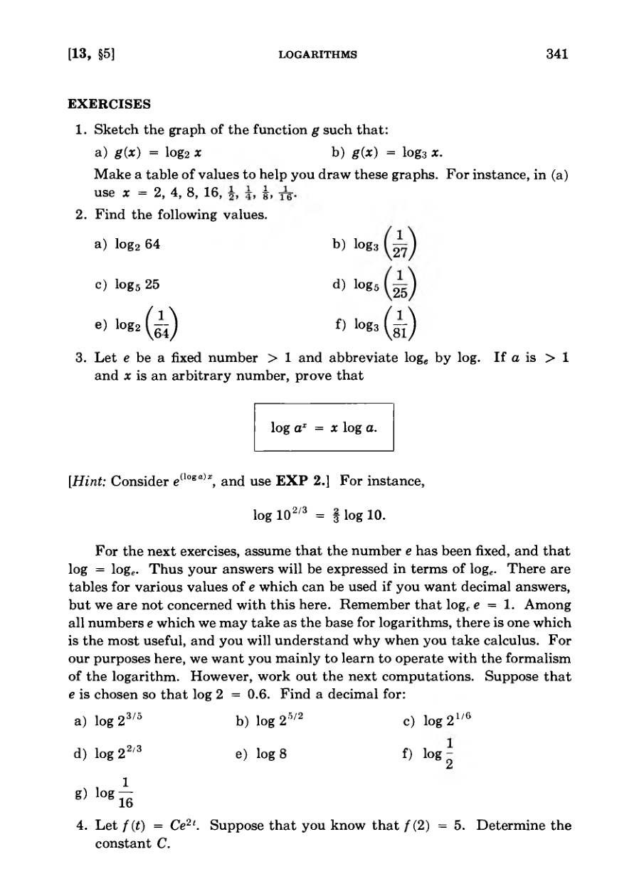
Provides exercises for sketching logarithmic graphs and evaluating logarithmic values.
Explores the properties and formalism of logarithms with a fixed base e.
Applies exponential and logarithmic formulas to real-world problems involving radioactive decay.
Models population growth and bacterial increase using mathematical constants.
Observe how in this example the unspecified constant C does not appear in the final answer.
Diagram
Defining Mathematical Mappings
A mapping is defined as a general association between elements of two sets, extending the concept of functions.
Functions and geometric transformations are both specific examples of mappings between sets.
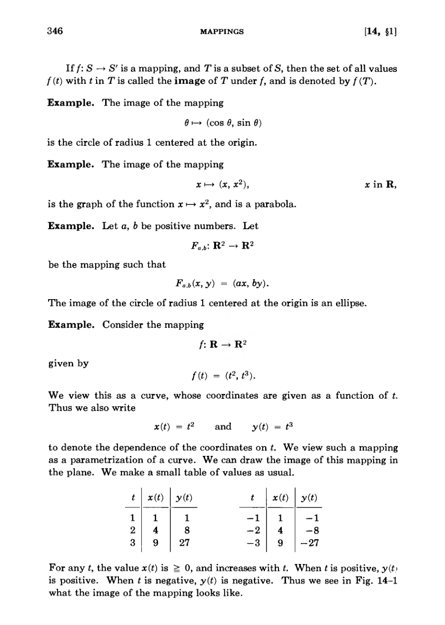
Mappings can be used to describe parametric equations of lines and circles in the plane.
The image of a subset under a mapping represents the set of all resulting output values.
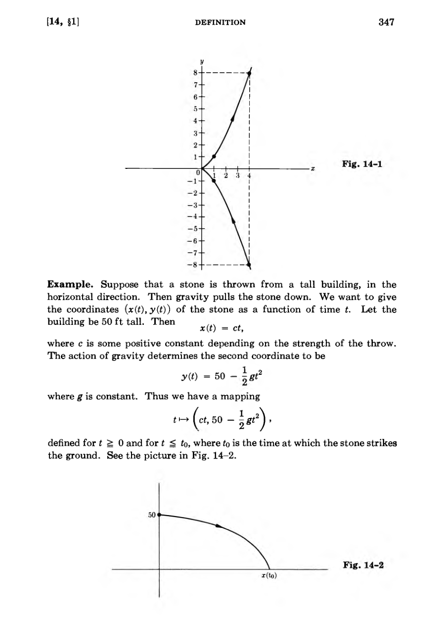
Physical phenomena, such as a stone thrown from a building, can be modeled using mappings of time to coordinates.
We note that a function is an association.
TableFigure
Mappings and Functions
A mapping from any set into the real numbers is formally defined as a function.
Distance functions assign to each point its numerical distance from a designated origin or another point.
Functions can represent physical quantities like temperature changing over time.
Exercises explore the graphical images of various mappings from real numbers into a two-dimensional plane.
Several problems model physical scenarios, such as projectiles and particles, whose coordinates are functions of time.
The polar coordinate map transforms geometric regions like rectangles into circular sectors.
A particle starts from a point (0, 6) in the plane. It is attracted by a magnet along the jc-axis, and repelled by a magnet along the y-axis in such a way that its coordinates are given by...
Formalism and Composition of Mappings
Mappings satisfy a general formalism that includes the identity mapping, which leaves every element unchanged.
Composite mappings are formed by applying one mapping after another, provided the codomain of the first is a subset of the domain of the second.
Composition of mappings is associative, meaning the grouping of successive mappings does not affect the final result.
The identity mapping behaves analogously to the number one when composition is treated like multiplication.
Inverse mappings undo the effect of a given function and are unique when they exist.
Mappings can be iterated multiple times, leading to an exponential notation for repeated applications.
We note that the identity mapping behaves like the number 1 in a context where composition of mappings behaves like multiplication.
Formalism and Iteration of Mappings
Iterating linear functions and translations reveals predictable patterns where applying a function k times adds a multiple of its constant or vector.
Functions like powers of x demonstrate exponential growth under repeated iteration, such as f^k(x) = x^(3^k).
The general rule of exponents for mappings states that f^(m+n) equals the composition of f^m and f^n, which holds for positive, zero, and negative integers.
Negative integer exponents are defined using the inverse mapping f^(-1) composed with itself k times, acting analogously to algebraic inverses.
Proofs involving integer exponents can be formalized and rigorously established using mathematical induction.
Observe again how composition of mappings is analogous to multiplication.
Figure
Mappings and Permutations
The text introduces the cancellation law for mappings, demonstrating that if compositions are equal and an inverse exists, the underlying mappings must be equal.
A series of exercises explore properties of specific mappings on coordinate spaces and general sets, requiring proofs of invertibility and algebraic manipulation of map powers.
The concept of permutations on a finite set of integers is defined as an injective and surjective mapping of the set onto itself.
Permutations can be composed to form a product, and examples demonstrate that this operation is generally not commutative.
The notation for permutations represents the rearrangement of elements in a sequence, highlighting the unique preimage for each element in the codomain.
Watch out! It is not always true that <j<j' = a'a.
DiagramDiagramDiagram
Inverse and Transposition Permutations
Inverse permutations reverse the mapping of original permutations such that their composition yields the identity permutation.
The inverse of a composite permutation reverses the order of the individual permutations in the product.
A transposition is a specific type of permutation that interchanges two distinct numbers while leaving all others fixed.
Every permutation of a finite set can be expressed as a product of transpositions through a systematic reduction procedure.
The identity permutation can be correctly interpreted as the product of zero transpositions under a standard mathematical convention.
Just multiply one with the other, and you will find that all the factors cancel out to give the identity.
DiagramFigure
Parity of Permutations
While the expression of a permutation as a product of transpositions is not unique, a fundamental consistency remains.
Theorem 2 states that any permutation can be classified by the parity of its transpositions as either always even or always odd.
An even permutation is expressed as a product of an even number of transpositions, yielding a sign of positive one.
An odd permutation requires an odd number of transpositions, resulting in a sign of negative one.
Applying successive powers of a permutation to a finite set element eventually reveals a repeating cycle.
The smallest positive integer mapping an element back to itself defines the distinct cycle length for that element.
In any expressions of a as a product of transpositions, the number of transpositions occurring in such a product is either always even or always odd.
FigureDiagram
Permutation Orbits and Cycles
An orbit of a permutation consists of a set of elements generated by repeatedly applying the permutation to a starting element.
The sequence of elements in an orbit forms a cycle, and the number of elements in this cycle is defined as the period or length.
Different starting elements within the same orbit can generate cyclically equivalent representations, such as [1, 3, 4] and [3, 4, 1].
Theorem 3 establishes that any two orbits of a permutation either completely coincide or are entirely disjoint.
Every permutation can be uniquely expressed as an orbit decomposition, which is a product of its disjoint cycle components.
Theorem 3. If a, b are elements of J n and a is a permutation of J n, then the orbits to which a and b belong either coincide, or have no element in common, i.e. are disjoint.
DiagramDiagramDiagramFigure
Orbits and Permutation Parity
Analyzing how a transposition affects permutation orbits divides into two distinct cases based on whether the elements belong to the same orbit or different orbits.
When a transposition acts on elements within the same orbit, it splits that orbit into two distinct pieces, increasing the total number of orbits by one.
Conversely, when a transposition acts on elements in different orbits, it merges them into a single orbit, thereby decreasing the total number of orbits by one.
Applying these rules successively proves that a permutation cannot be expressed as both an even and an odd number of transpositions.
Theorem 4 establishes a clear rule for permutation parity: if n minus the number of orbits is even, the permutation is even, and if odd, it is odd.
However the integer (Number of orbits of <r) — n is either odd or even, and cannot be both.
Permutations and Complex Numbers
Exercises involve expressing permutations as products of transpositions and determining their signs.
Problems require finding the inverse and orbit decomposition for various permutations.
Proofs demonstrate properties such as the equal distribution of odd and even permutations.
Induction proves that the total number of permutations of a set of size n is equal to n factorial.
The text introduces complex numbers as a system where addition and multiplication satisfy standard algebraic properties.
Complex numbers are defined to include a special element i whose square is minus one, and can be geometrically represented in a plane.
There exists a complex number i such that i2 = —1.
FigureFigure
Properties of Complex Numbers
Complex numbers can be defined and multiplied algebraically, leading to the rule that the product of points (x,y) and (u,v) is (xu-yv, xv+yu).
Real numbers are identified as points of the form (a,0) in the complex plane, using the fundamental rule that i squared equals negative one.
The complex conjugate of z = a + bi is defined as z-bar = a - bi, and the product of a number and its conjugate yields the squared distance from the origin.
Every non-zero complex number possesses a unique multiplicative inverse constructed using its conjugate and absolute value.
The absolute value of a complex number represents its geometric distance from the origin, satisfying properties such as the triangle inequality.
This would be boring, so we omit it, and just assume all the properties.
Figure
Polar Form of Complex Numbers
Complex numbers can be represented geometrically in the plane using polar coordinates.
Every complex number can be expressed in polar form as the product of a real number and a complex number with an absolute value of 1.
Euler's formula defines complex exponentials using sine and cosine functions.
Multiplying complex numbers in polar form involves multiplying their absolute values and adding their angles.
Complex exponentiation obeys the same basic algebraic rules as ordinary exponentiation.
Thus, to multiply complex numbers, we may say roughly that we multiply their absolute values and add their angles.
Diagram
Mathematical Induction and Summations
Induction is an axiom used to prove that mathematical properties hold true for all positive integers.
The proof process requires establishing a base case (IND 1) and proving that if the assertion holds for n, it holds for n + 1 (IND 2).
Sigma notation (capital Greek sigma) provides a concise way to write sums without using intermediate dots.
Mathematical induction can be applied to prove formulas for sums of integers, functional behaviors, and binomial coefficients.
Binomial coefficients, denoted as C_n^k, represent the number of ways to select k objects out of a set of n objects.
IND 1 gives us a starting point, and IND 2 allows us to prove A(2) from A(1), then A(3) from A(2), and so forth, proceeding stepwise.
Mathematical Induction and Summations
The text provides a series of mathematical exercises focusing on proof by induction, formulas for sums of powers, and properties of functions.
It introduces binomial coefficients and asks students to prove fundamental assertions regarding them.
A famous fallacious proof by induction is presented, challenging students to find the flaw in the argument that all billiard balls have the same color.
The second section transitions into summations, applying them to ancient geometric problems of computing volumes of solids of revolution.
Archimedes' method is introduced to approximate the volume of a cone by dividing it into a series of cylindrical slices.
Theorem. All billiard balls have the same color.
DiagramDiagram
Calculating Cone Volumes
The volume of a specific cone is determined by summing the volumes of small approximating cylinders and taking the limit as the number of partitions increases.
Using algebraic expressions for sums of squares allows the limit to be evaluated cleanly to find the volume of a unit cone.
Arbitrary cones can be analyzed either by repeating the limiting process with generalized dimensions or by applying mixed dilations.
A mixed dilation scales the coordinates in three dimensions independently, multiplying the volume of any solid by the product of the scaling factors.
Applying the mixed dilation factor of abc equal to hr2 to the base cone yields the classic volume formula for any cone with radius r and height h.
In other words, the volume gets multiplied by abc under the mixed dilation.
DiagramDiagramFigureDiagramDiagram
Geometric Series and Cones
Cones can be transformed and understood as images under mixed dilations.
Exercises explore volumes of solids of revolution and areas under curves using approximations.
The finite sum of a geometric series simplifies using algebraic distributivity.
As the exponent grows, powers of fractions strictly less than one approach zero.
Infinite geometric series converge to a specific limit given by the formula 1 divided by 1 minus c.
There is no number called “ infinity” .
Figure
Mathematical Induction And Summations
Exercises explore the numerical values of geometric series for various specific numbers.
Problems extend geometric series concepts to complex numbers within the unit disk.
Summations involving powers of roots of unity are investigated.
A 2 by 2 matrix is an array of four numbers that can be viewed as a generalization of pairs.
Matrices can be analyzed through their horizontal rows or vertical columns.
Pairs of numbers written vertically or horizontally are defined as vectors, categorized as column or row vectors.
In this way, show that these sums can be made to have arbitrarily large values, for sufficiently large n.
Diagram
Matrices and Determinants
Matrices are numerical arrays denoted by subscript indices for rows and columns, generalized here for 2x2 and 3x3 dimensions.
Transposition of a matrix involves flipping it across the diagonal, changing rows into columns while keeping diagonal components unchanged.
The determinant of a 2x2 matrix is defined as the number calculated by the expression ad minus bc.
Determinants serve as crucial mathematical tools for determining the unique solvability of systems of linear equations.
The proof for linear equation solutions relies on algebraic elimination of variables using the non-zero condition of the determinant.
The determinant is an important tool for solving linear equations.
DiagramDiagramDiagram
Properties of 2x2 Determinants
Algebraic verification confirms that formulas involving determinants correctly solve systems of two linear equations.
Determinant solutions express unknowns as quotients of smaller determinants, demonstrating a clear structural pattern.
While elimination is often easier for 2x2 systems, determinants provide a foundation for handling more unknowns.
Theorem 2 establishes that the determinant of a 2x2 matrix equals the determinant of its transpose.
Determinants exhibit column-based properties, notably satisfying distributivity with respect to vector addition.
Note how the column occurs as the first column in the numerator for x, and how it occurs as the second column in the numerator for y.
Diagram
Properties of 2x2 Determinants
Fundamental properties like D3 and D4 serve as the basis for deriving other determinant rules without relying on raw matrix components.
Property D5 demonstrates that adding a multiple of one column to another leaves the determinant's value unchanged.
Property D6 shows that interchanging columns reverses the sign of the determinant, proving that the operation is anti-commutative.
Abstract proofs using foundational properties scale better to higher dimensions than messy component-based calculations.
Systems of linear equations can be solved efficiently using determinant properties to isolate variables like x and y as quotients.
Observe that D6 shows that our determinant, viewed as a “ product,” is not commutative.
Determinants of Order Three
The text introduces the definition of determinants for 3 x 3 matrices using expansion by a row.
Determinants can be computed by multiplying elements of a row by the determinants of smaller 2 x 2 submatrices with alternating signs.
Expanding a determinant along different rows or columns consistently yields the same numerical value.
Strategic choice of rows or columns containing zeros can simplify determinant calculations by eliminating terms.
Theorem 3 establishes that the determinant of a matrix is equal to the determinant of its transpose.
Note that the presence of 0 in the first row and second column eliminates one term in the expansion, since this term is equal to 0.
DiagramDiagramFigure
Properties of 3x3 Determinants
Provides a series of practice exercises for computing 3x3 determinants using different expansion rows and columns.
Explores formulas for evaluating special determinants involving parameters and triangular matrices.
Introduces fundamental properties D1 through D4 for 3x3 determinants, focusing on column operations.
Demonstrates that a determinant splits into a sum when one of its columns is expressed as a sum of two vectors.
Shows that scalar multiplication of a column scales the entire determinant by the same factor.
Establishes that determinants equal zero when any two columns are identical and confirms the unit matrix determinant is one.
If two columns of the matrix are equal, then the determinant is equal to 0.
FigureDiagramDiagramDiagram
Properties of Determinants
Remaining determinant properties, such as D5 and D6, can be proven using only the formalism of D1 through D4 rather than direct row expansion.
Property D5 states that adding a multiple of one column to another does not change the determinant's value.
Property D6 dictates that interchanging two adjacent columns causes the determinant to change by a sign.
These formal properties allow for much more efficient computation of determinants by strategically introducing zeros.
Using elementary column or row operations simplifies complex matrix evaluations down to manageable single-term expansions.
If two adjacent columns are interchanged, then the determinant changes by a sign.
DiagramFigureDiagram
Cramer's Rule for Linear Equations
Exercises explore properties of determinants, including linearity with respect to column additions.
Linear equations in three unknowns can be expressed compactly using vector and matrix notation.
Theorem 4 introduces Cramer's rule, providing explicit determinant formulas for the variables when the determinant is non-zero.
The text notes that Cramer's rule assumes a solution exists rather than proving existence on its own.
Theorem 5 establishes that a solution indeed exists for any column B if the coefficient matrix determinant is not zero.
An explicit numerical example demonstrates how Cramer's rule is applied to solve a specific system of three linear equations.
Observe that Theorem 4 does not tell us that a solution exists.
DiagramFigure
Determinants and Mathematical Index
The text illustrates how column positions shift when solving for different variables using Cramer's rule.
The denominator remains consistent across expressions as the determinant of the coefficient matrix.
Exercises prompt the reader to prove Cramer's rule for specific variable sets and solve linear equations.
A comprehensive alphabetical index covers mathematical concepts ranging from absolute value to zero.
Entries in the index reference foundational topics such as algebra, geometry, permutations, and trigonometry.
Observe how the column shifts from the first column when solving for x, to the second column when solving for y, to the third column when solving for z.
Diagram
Answers to Selected Exercises
The text provides solutions to mathematical exercises from Chapter 1, sections 2, 3, and 4.
Proofs demonstrate algebraic properties such as associativity and commutativity for addition and subtraction.
Expansions of binomial cubes and higher powers are solved step-by-step.
Parity proofs show the algebraic behavior of even and odd numbers under addition and multiplication.
Modular arithmetic problems illustrate divisibility and equivalence relations.
Step-by-step derivations validate cancellation laws and equations involving variables.
It suffices to show that (a + b + c) + ( —a) + ( —6) + ( — c) = 0.
Selected Mathematical Exercises and Proofs
The text provides answers and step-by-step solutions to selected mathematical exercises from various chapters.
Proofs regarding the divisibility of numbers by three and the irrationality of cube roots of certain integers are detailed.
Algebraic manipulations demonstrate polynomial factorizations and rational expressions.
Factorial calculations and combinatorial formulas are also included in the problem sets.
Approximations and numerical values are provided for various algebraic and arithmetic problems.
Thus both m and n are even, which is impossible.
Selected Mathematical Exercise Answers
The text provides solutions to mathematical problems and exercises across various chapters and sections.
Answers include numerical values for variables such as x, y, and z in algebraic equations.
Temperature conversions and physical measurements like volume and weight are listed as problem solutions.
Detailed proofs and step-by-step arithmetic manipulations demonstrate how to handle inequalities and positive numbers.
Explanations cover properties of square roots, exponents, and rational versus irrational numbers.
This is impossible since Vx cannot be negative.
Selected Exercise Answers
The text provides answers and step-by-step proofs for selected mathematical exercises.
Inequalities are proven and manipulated through algebraic methods like cross multiplication.
Solutions to various algebraic equations and problems involving real numbers are listed.
Calculations of areas, angle measurements, and geometric properties are presented.
Distance formulas and triangle theorems are verified through coordinate geometry and proofs.
Impossible with real numbers, (4 +- V -4)/2
DiagramDiagram
Selected Mathematical Exercises Solutions
Provides step-by-step solutions for geometric area calculations involving triangles.
Applies the Pythagorean theorem to analyze distance relationships between points.
Demonstrates angle equalities using right triangles and perpendicular properties.
Lists fixed points for various geometric transformations including reflections and rotations.
Explains that isometries preserve distances and map parallel lines to parallel lines.
All points of the plane are fixed.
DiagramDiagramDiagram
Theorem Proofs and Exercise Answers
Theorem 4 establishes that an isometry in three-space is the identity if it fixes four non-coplanar points.
The proof constructs intersecting planes and lines to demonstrate that any arbitrary point in space remains fixed under the isometry.
Selected exercise answers demonstrate properties of isometries, including inverses, compositions, and congruent sets.
Mappings such as translations and rotations are used to reduce complex geometric proofs to simpler cases.
Cayley tables and permutation matrices are provided for specific algebraic structures and group operations.
Theorem 4. If P, Q, R, S are four points which do not lie in a plane and are fixed by an isometry f of 3-space, then f is the identity.
DiagramDiagramDiagram
Selected Geometric Solutions
Demonstrates the use of isometries and reflections to prove the coincidence of squares with identical corners.
Applies angle theorems on right triangles to show that specific sides maintain equal lengths through reflection.
Solves various exercises involving coordinate geometry, distance formulas, and geometric transformations.
Computes areas and volumes under linear dilations, showing scaling relationships.
Provides numerical answers for selected exercises spanning multiple chapters of geometry.
This is the set of all line segments PQ, where P lies on one side of the square and Q lies on the other.
DiagramDiagramDiagram
Selected Mathematical Exercises Solutions
The text provides answers to selected mathematical exercises, primarily covering chapters on inequalities and coordinate geometry.
Calculations demonstrate properties of translations, reflections, and distances between points in a coordinate plane.
Algebraic manipulations confirm relationships between vectors, line segments, and geometric transformations.
Conditions for parallelism of vectors and lines are derived using determinants and cross-multiplication.
Formulas for reflections through points and circles illustrate invariant properties under rigid motions.
A and B are parallel if and only if A = cB, with some number c not equal to 0; that is, (a1, a2) = (cb1, cb2).
DiagramChart
Selected Mathematics Exercises Answers
The text provides answer keys for selected exercises from mathematical chapters involving analytic geometry and trigonometry.
Comprehensive tables list sine, cosine, and tangent values for various multiples of pi over six and pi over four.
Algebraic derivations show the intersection points between lines and circles using quadratic equations.
Trigonometric identities and angle conversions are systematically presented across multiple chapters and sections.
Numerical solutions for applied geometry problems, such as heights and distances, are detailed.
The line is described by (p + at, q + bt), t in R.
ChartDiagramDiagram
Trigonometry and Calculus Answer Key
The text provides mathematical identities involving trigonometric functions such as sine and cosine.
Selected answers for exercises span multiple chapters covering advanced topics like coordinate geometry and functions.
Algebraic manipulations are detailed for solving systems of linear and parallel equations.
Properties of geometric conic sections including centers and extremities are listed for various chapters.
Function definitions, parity tests for odd and even functions, and composite mappings are evaluated.
If they are parallel, then a = c. Any point (x, y) in common would be such that ax + b = ax + d, so b = d which is impossible.
DiagramDiagramDiagramDiagramDiagram
Selected Textbook Answers
The text provides answers to selected mathematical exercises spanning multiple chapters.
Calculations involve polynomial degrees, roots, rational functions, and exponential expressions.
Parametric equations and their corresponding geometric curves are evaluated.
Function composition, inverses, and functional relationships are analyzed.
Permutations, transpositions, and their signs are computed in later sections.
The ray is open, i.e. does not contain the origin, because for all numbers y , the number 2y is > 0!!
DiagramGraphDiagramGraphDiagramDiagramDiagram
Selected Mathematics Exercise Answers
Provides answers and proofs for selected permutation exercises involving even and odd permutations.
Demonstrates mathematical induction to calculate the total number of permutations in Sn+1.
Solves various problems related to complex numbers, including conjugates, imaginary parts, and roots.
Uses Euler's formula to derive expressions for cosine and sine functions.
Applies mathematical induction to prove algebraic identities and sequence formulas.
Adding the two equations yields e^(i\theta) + e^(-i\theta) = 2 \cos \theta.
Selected Exercise Answers
The text provides solutions and selected answers to mathematical exercises across various chapters.
Early sections cover algebraic expansions, induction proofs, and binomial coefficients.
Calculus applications such as volume estimation using cylindrical segments are solved in later chapters.
Series convergence tests and limit calculations are demonstrated with explicit steps.
Linear algebra topics including determinants and properties of functions are detailed with step-by-step proofs.
There is no “middle” ball!!
Diagram
Answers and Author Biography
Provides mathematical solutions and proofs concerning determinants and row operations in Chapter 17.
Demonstrates properties of determinants such as invariance under row additions and sign changes under row interchanges.
Calculates specific numerical values for determinants and solves linear combinations of vectors.
Details the academic background and prolific publishing history of mathematician Serge Lang.
Advertises related mathematics textbooks authored by Serge Lang, covering calculus and linear algebra.
If you add a multiple of one row to another, you do not change the value of the determinant.
New Book Edition Updates
New examples and exercises have been added to the current edition.
The first half of the book underwent extensive revision by the author.
New material covers unitary maps over the reals.
Content on the Jordan canonical form has been introduced.
The spectral theorem is now included as part of the new material.
New material on unitary maps over the reals, the Jordan canonical form, and spectral theorem has also been introduced.
Kept 139 of 139 sections, 59 of 584 figures.
Rules of Number Operations
Many algebraic properties, such as commutativity and associativity, apply broadly to other mathematical objects like functions and mappings.
The whole first part on algebra is much more dry than the rest of the book, and it is good to motivate this algebra through geometry.
Extending Number Systems
Mathematical systems often expand to allow equations to be solved that were impossible in smaller systems.
This pattern is related to the extension of one system of objects to a larger system, in which more equations can be solved than in the smaller system.
Adding Negative Numbers and Integers
The term 'minus a' is preferred over 'negative a' because -a is not necessarily negative unless a is positive.
I find the words “negative a” confusing, because they suggest that —a is a negative number.
Rules of Addition
Numbers and their negatives occur symmetrically on opposite sides of zero on the number line.
In the geometric representation of numbers on the line, a and —a occur symmetrically on the line on opposite sides of 0.
Rules for Multiplication
Operating with negative numbers follows rigorous laws, including the principle that the product of two negatives is a positive.
This is one of the most frequent sources of error when we work with multiplication and addition.
Rules for Multiplication and Powers
Three fundamental algebraic formulas for squaring binomials and finding the difference of squares are introduced and proven using multiplication rules.
They are so important that they should be thoroughly memorized by reading them out loud and repeating them like a poem to get an aural memory of them.
Even and Odd Integers
An even integer can be expressed algebraically in the form 2n, while an odd integer can be written as 2n + 1 or 2m - 1.
Thus the odd integers go up by 2 and the even integers go up by 2.
Divisibility and Rational Numbers
Fractions lack a unique representation, leading to the rule of cross-multiplying to determine when two expressions yield the same rational number.
There is no unique representation of a rational number as a quotient of two integers.
Rational Numbers and Cancellation
The cancellation rule demonstrates that multiplying or dividing the numerator and denominator by the same non-zero integer preserves the fraction's value.
Some people view this proof as the reason why cross-multiplication works.
Adding and Multiplying Fractions
The addition of rational numbers with a common denominator is derived naturally from the meaning of fractions.
If we have three-fifths of something, and add eight-fifths of that same thing, then we get eleven-fifths of that thing.
Multiplying Fractions and Square Roots
Despite getting arbitrarily close through approximations, a rigorous mathematical theorem proves that no positive rational number actually has a square of 2.
However, to find a rational number whose square is 2, the procedure is a bummer because of the following theorem.
Rational Numbers and Equations
The proof that the square root of two is irrational concludes by showing that an original assumption leads to a contradiction.
Thus from our original assumption that (m/n)2 = 2 and m/n is in lowest form, we have obtained the impossible fact that both m, n are even.
Rational Numbers and Multiplicative Inverses
Word problems involving chemical decay, bacterial populations, and lake pollution illustrate exponential decrease and fractions of remaining substances over time.
A chemical substance decomposes in such a way that it halves every 3 min.
Rational Numbers and Fractions
Cross-multiplication states that if a/b = c/d, then ad = bc, and vice versa, proven using basic field properties.
Thus we can operate with fractions formed with rational numbers much as we could operate with fractions formed with integers.
Algebraic Word Problems and Proofs
Practical applications are demonstrated through word problems involving travel speed and mixture concentrations.
A person takes a trip and drives 8 hr, a distance of 400 mi.
Solving Linear Equations
The elimination method is demonstrated by multiplying equations to make coefficients of one variable match.
We try to get rid of x, say, so as to obtain only one equation in y.
Solving Linear Equations
Simultaneous equations correspond to finding the intersection point of straight lines in coordinate geometry.
We don’t intend to overburden you or give you any worries about them.
Solving Linear Equations
Strategic ordering of equations during elimination makes the algebraic process significantly easier.
We choose the order of elimination so as to make it easier on ourselves.
Real Numbers Properties and Positivity
Systems with only two objects, such as even and odd abstractions, can satisfy these same basic arithmetic properties.
Thus real numbers are not the only system to satisfy these properties.
Positivity and Square Roots
Every positive real number is assumed to have a square root, proving the existence of irrational numbers like the square root of two.
Because of this, and Theorem 4, §5 of Chapter 1, we now see that a number whose square is 2 is irrational, but exists as a real number.
Rationalizing Square Roots
Advanced calculus techniques often require rationalizing the numerator to transform expressions into more workable forms.
This example has the same notation as an actual case which arises in more advanced courses of calculus.
Powers and Roots
The n-th root of a positive real number is defined as the unique positive real number r whose n-th power equals a.
Let a be a positive number and let n be a positive integer. As part of the properties of real numbers, we assume, but do not prove, that there exists a unique positive real number r such that rn = a.
Real Numbers and Inequalities
Multiplying both sides of an inequality by a negative number reverses the direction of the inequality.
Rule IN 3 tells us that if we multiply both sides of an inequality by a negative number, then the inequality gets reversed.
Proving Inequalities and Intervals
Solving inequalities with variables in the denominator requires splitting the domain into separate cases.
Note that the quotient on the left makes no sense if x = 4.
Real Numbers and Quadratic Equations
Examples illustrate that some quadratic equations yield multiple real solutions while others have no solutions in real numbers.
But a negative real number cannot possibly be a square of a real number and we conclude that our equation does not have a solution in real numbers
Deriving The Quadratic Formula
The quadratic formula should be memorized thoroughly, even by reading it aloud like a poem.
Read it out loud like a poem, to get an aural memory of it: “x equals minus b plus or minus square root of b squared minus four ac over two a.”
On Reading Mathematics Books
Books must be organized linearly on pages, which distorts the natural simultaneity of how the human brain perceives ideas.
In writing the book, the whole subject has to be organized in a totally ordered way, along lines and pages, which is not the way our brain works naturally.
Mathematical Logic and Converse Statements
Proof by contradiction establishes the truth of a statement by showing that its negation leads to an absurdity.
We want to prove that a certain statement A is true.
Mathematical Language and Sets
Equality strictly means that two expressions refer to the exact same object.
We DO NOT USE THE WORD “ EQUALITY” AS IT IS SOMETIMES USED, for instance in elementary geometry.
Mathematical Notation and Sets
Mathematical conventions allow variables like x and y to be equal unless explicitly stated otherwise as distinct.
It is clear that we would soon run out of letters of the alphabet in enumerating numbers just with letters, and hence we use a notation with subscripts...
Mathematical Notation and Intuitive Geometry
While notation should be clear, authors must navigate a limited alphabet and occasional imperfections by encouraging active learning.
If you find any such things in the present book, then correct them or improve them for yourself, or write your own book.
Analytic Foundations of Geometry
Historical progress in mathematics was long hindered by an unnecessary inhibition against applying numbers to geometric objects.
One reason why the Greeks did not get further in their mathematics is that they suffered from the inhibition of using numbers to deal with geometric objects.
Foundations of Geometric Measurement
Angles are defined as regions of the plane separated by two rays sharing a common vertex rather than simply the union of the rays.
They do not think neutrally.
Defining Angles and Arcs
Ordering the rays determines a specific angle by following the counterclockwise direction from the first ray to the second.
Just knowing the two rays is not enough information to be able to distinguish one angle from the other.
Measuring Angles with Degrees
The degree measure of an angle is defined through the ratio of the area of its sector to the total area of the disc.
In computing the number of degrees in an angle, we do not have to determine the area of S or even that of D, only the ratio between the two.
Geometry Exercises and Triangles
The author discusses terminological ambiguity surrounding whether a triangle refers to its boundary or the enclosed region.
Nobody will accept 'trisc'.
Axioms of Geometry and Pythagoras
Geometric theory balances minimizing basic assumptions with maximizing easily deduced properties that feel intuitively obvious.
If I didn’t think that the choice I have made about this was reasonably successful, I wouldn’t have written a book . book . . .
Geometry of Rectangles and Triangles
Introduced the Pythagorean theorem, relating the lengths of the legs and the hypotenuse of a right triangle.
We are committing here the same abuse of language by speaking of the area of the rectangle that we did with triangles.
The Pythagorean Theorem
Properties of the perpendicular bisector of a line segment are defined and proven using distance equations.
Observe that if O is any point on the line passing through P and Q which is such that d(O,P) = d(O,Q), then O is necessarily on the segment between P and Q.
Geometry Exercises and Isometries
Introduces the concept of congruence through visual examples like discs and triangles.
Roughly speaking, this means that one figure can be laid over the other.
Standard Mappings in Geometry
Dilations stretch or shrink distances from a fixed point by a positive scale factor r.
A dilation is also sometimes called a similarity transformation, but the word dilation is the shortest and best term to be used to denote the concept.
Defining Geometric Rotations
A 180-degree rotation around a center point is mathematically equivalent to a reflection through that same point.
Observe that rotation by 180° with respect to O is none other than reflection through O.
Understanding Plane Isometries
An isometry is defined as a mapping of the plane into itself that strictly preserves the distances between every pair of points.
Let F be a mapping of the plane into itself. We say that F preserves distances, or is distance preserving, if and only if for every pair of points P, Q in the plane, the distance between P and Q is the same as the distance between F(P) and F(Q).
Properties of Isometries
Proving set equality in the theorem follows a standard mathematical pattern by showing each set is contained within the other.
In this proof, we want to show that two sets of points are equal.
Theorem 3 and Composition of Isometries
The proof constructs intersecting lines through fixed points to demonstrate that any arbitrary point must also be fixed.
We can find a line L passing through X which intersects LPQ in a point Z, and intersects LQM in a point Y such that Y != Z.
Composition of Isometries
Iterating an isometry multiple times creates powers that mirror algebraic exponent rules like F^(m+n) = F^m o F^n.
Note this interesting cyclical nature of F, that F5 = F.
Geometry and Isometry Exercises
Exercises involve applying reflections, rotations, and their compositions to points in the plane.
Draw a small flower. Let T be translation by 1 in. to the right, and let U be translation by 1 in. vertically upward.
Inverse and Equality of Isometries
A corollary to Theorem 3 demonstrates that if two isometries map three non-collinear points to the same locations and an inverse exists, the isometries are identical.
Using inverses, we can now prove a very useful corollary of Theorem 3 which tells us when two isometries are equal.
Multiplication Tables and Isometries
Introducing the characterization of isometries as composites of translations, rotations, and reflections.
The main result of this section is that an isometry can be expressed as a composite of a translation, a rotation, and possibly a reflection.
Characterization and Congruence of Isometries
Theorem 6 classifies an arbitrary isometry without fixed points as a translation, a translation combined with a rotation, or further combined with a reflection.
If F does not leave any point fixed, then F is either a translation, or the composite of a translation and a rotation, or the composite of a translation, a rotation, and a reflection through a line.
Geometric Congruence Proofs
Reflections and perpendicular bisectors are utilized to map remaining points and complete the ultimate triangle congruence proof.
Hence if we reflect M' through Lpq, we get M.
Geometrical Shapes And Isometries
Isometries preserve the measure of angles, though reflections have the specific property of reversing the order of the rays used to compute that measure.
Note, however, that a reflection reverses the order of the rays which are used to compute the measure of the angle in counterclockwise direction.
Area and Dilation
Using this principle, the area of a disc of radius r is expressed as pi times r squared, where pi represents the numerical area of a disc of radius one.
It is of course a problem to determine its numerical value.
Approximating Area with Grids
By making the grid finer, the total area of the boundary-touching squares becomes vanishingly small.
We have a very strong intuition that the sum of such little squares will be quite small if our grid is fine enough, and in fact, we give an estimate for this smallness in the following discussion.
Dilation and Circle Circumference
To study the length of a curve like a circle, the text transitions from approximating areas with squares to approximating curves with straight line segments.
To study length, we have to approximate a curve by means of straight line segments.
Circle Area and Dilation
By taking the limit as sides increase, the classic formula for the circumference of a circle is derived.
As n becomes arbitrarily large, An approaches the area of the disc Dr, Pn approaches the circumference of the circle Cr, and hn approaches the radius r of the disc.
Introduction to Coordinate Geometry
Part Three introduces coordinate geometry as a method to translate geometric terms into numerical properties.
Giving coordinates to points not only allows us to give analytic proofs.
Introduction to Coordinate Systems
Coordinate systems are flexible and can even be represented using slanted axes or applied to map geographical locations.
View the distortion in the same spirit as you view modern art.
Coordinates and Distance Geometry
A continuous big exercise challenges students to extend two-dimensional geometric concepts into three-dimensional space.
Write it all up as if you were writing a book. This will make you really learn the subject.
Distance Between Points
The plane is formally defined as the set of all pairs of real numbers to build geometry upon number properties.
Warning: Always be careful when you meet minus signs.
The Equation of a Circle
Squaring both sides of the distance equation helps avoid messy square root signs in standard circle equations.
It is often convenient to leave the equation of the circle in the form, to avoid writing the messy square root sign.
Rational Points On Circles
By dividing the equation by c squared, the problem of finding integer right triangles is transformed into finding rational points on the unit circle.
The result proved in this section is not essential for what follows, and may be skipped. It is, however, quite beautiful.
Rational Points On Circles
Mathematical talent is distinguished by the ability to discover such beautiful formulas rather than merely plugging numbers into them.
What distinguishes someone with talent for mathematics from someone without talent is that the first person will be able to discover such beautiful formulas and the second person will not.
Dilations and Reflections of Points
Multiplying a point by a real number scales its coordinates by that factor, a geometric process known as dilation.
Geometrically, we see that multiplication by 3 stretches the coordinates by 3.
Operations on Points
Geometric interpretation reveals that points O, A, B, and A + B form the corners of a parallelogram.
Thus the four points O, Ay By A + B form the four corners of a parallelogram, which we draw in Fig. 9-6 (c).
Geometric Translations and Norms
Geometric notions like distance and translation are successfully expressed using purely numerical properties.
We see that we have been able to define one more of the intuitive geometric notions within our system of coordinates, based only on properties of numbers.
Operations and Transformations on Points
Ordinary arithmetic rules for numbers, such as associativity and distributivity, apply directly to the addition and multiplication of points.
We ask whether the ordinary rules which we had for numbers also apply, and the answer is yes.
Mapping Exercises and 3-Space
Extends 2-dimensional concepts of points, translations, and isometries into 3-space and higher dimensions.
And higher. Why not?
Writing Mathematics and Segments
Copying mathematical theory between dimensions or from experts is a historically valid learning technique, akin to Bach copying Vivaldi.
Do you know one of the means Bach used to learn how to compose? He copied practically the entire works of Vivaldi.
Understanding Rays and Directions
Located vectors can represent physical phenomena such as forces acting on particles or wind acting on airplanes.
In physics, located vectors are very useful to represent physical forces.
Vectors and Lines in Space
Parallelism for located vectors is defined analytically using scalar multiples.
Let PQ and MN be located vectors such that P != Q and M != N.
Parametric Representation of Lines
The parameter t can be interpreted physically as time, representing the position of a moving particle or bug along the line.
One sometimes interprets the point P + tA as describing the position of a bug, or a particle, moving along the line with uniform speed, and we interpret t as the time.
Intersections of Lines
A negative discriminant in the quadratic equation indicates that the line and the circle do not intersect.
We see that the expression under the square root sign is negative, and hence there is no real value of t satisfying our equation.
Ordinary Equation of a Line
The text introduces the concept of converting parametric line representations into ordinary equations by eliminating the parameter t.
So far we have described a line in terms of a parameter t. We can eliminate this parameter t and get another type of equation for the line.
Understanding Radian Measure
Historical choices led to the frequent appearance of the constant two pi, which the author notes is slightly inconvenient.
Too late to change, however.
Defining Sine and Cosine
Using a unit circle of radius 1, the coordinates of any point become simply the cosine and sine of the corresponding angle.
Consequently, by definition, the coordinates of a point on the circle of radius 1 are (cos 0, sin 0) if 0 is the angle in radians.
Trigonometry and Polar Coordinates
Practical applications of trigonometry to measure distances using small-sized instruments.
The whole point in this example is that the angle theta can be determined with a very small-sized instrument.
Trigonometric Exercises and Graphs
Practical word problems apply trigonometric concepts to real-world scenarios involving boats, balloons, and triangles.
A boat B starts from a point P and moves along a straight river.
Behavior and Graphs of Trigonometric Functions
The tangent of the angle a line makes with the x-axis corresponds precisely to the slope of that line.
If you read about the slope of a straight line in the next chapter, you will observe that the tangent of the angle which the line makes with the jc-axis is precisely its slope.
Trigonometric Applications and Formulas
Trigonometry allows for indirect measurement of large objects like towers using known distances and angles.
Suppose we want to determine the height of a tower without climbing the tower.
Trigonometric Addition Formulas
Memorizing a select few core formulas allows for the efficient derivation of all other trigonometric identities.
Read these out loud and get an aural memory of them.
Trigonometric Identities and Rotations
The resulting transformation equations for rotation naturally introduce the concept of a 2 by 2 matrix.
An array of numbers like has a technical name: It is called a matrix (in fact a 2 X 2 matrix).
Matrix Multiplication and Analytic Geometry
Matrix multiplication defines linear transformations like rotations and dilations using 2 by 2 matrices.
This is something like a multiplication.
Understanding Line Slopes
Swapping the order of the two points does not change the calculated slope value.
Observe that it does not matter which point we call (x1,y1) and which one we call (x2,y2).
Lines and Circles Intersection
A negative value under the square root in the resulting quadratic equation indicates that the line and circle do not intersect.
If we followed the same procedure to solve for x as before, we would find in this case that the quadratic equation has no real solution because the number under the square root sign is negative.
The Geometry of Parabolas
Beyond analytic geometry, parabolic mirrors possess the unique optical property of reflecting incoming horizontal rays to a single focal point.
If one makes a mirror in the shape of a parabola, then any horizontal ray coming into the mirror gets reflected, and all these reflections meet at one point, called the focus F of the parabola.
Analytic Geometry of Ellipses
A mixed dilation applied to the unit circle transforms it into a new geometric figure known as an ellipse.
Hence the image of the circle defined by equation (1) is the set of points (u, v) satisfying equation (2).
Graphing the Hyperbola
Hyperbolas naturally model physical phenomena, such as forces inversely proportional to distance.
In physics we encounter cases where an object is repelled from the origin along a straight line, with a force whose magnitude is inversely proportional to the distance from the origin.
Rotation of Hyperbolas
The mathematical principle is established that a rotation commutes with a dilation, meaning dilating followed by rotation yields the same result as rotating followed by dilation.
Our intuition immediately tells us how to find (x, y ) : these coordinates are obtained by rotating (u, v) through an angle of — 7r/4.
Hyperbolas and Functions
Functions can also be defined arbitrarily, such as assigning zero to rational numbers and one to irrational numbers.
Let G be the function such that G(x) = 0 if x is a rational number, G(x) = 1 if x is not a rational number.
Algebraic Properties of Functions
Functions can be used to model real-world phenomena, such as historical population growth and subway fares.
In physical life, functions of numbers occur when we describe one quantity in terms of another.
Properties of Polynomial Roots
A polynomial of degree n must have a uniquely defined degree, meaning it cannot be represented by coefficient sets of varying lengths.
If the answer were YES, then it would be hopeless to define the degree, because in the example just written down, for instance, we would not know whether the degree is 5 or 6.
Uniqueness of Polynomial Coefficients
Excessive emphasis on factoring in elementary classes is discouraged in favor of systematic formulas.
It is very unusual that a polynomial can be factored with integral or rational roots, and I think much too much emphasis is placed on this kind of accident.
Polynomial Long Division
Each step in polynomial long division systematically eliminates the highest degree term through subtraction.
Note that even though the standard procedure of the example, which gives us q, r, is called “ long division” , in fact our procedure uses only multiplication and subtraction.
Polynomial Euclidean Algorithm
The Euclidean algorithm provides a proof that if a polynomial has a root c, it can be factored by (x - c).
We do not prove the Euclidean algorithm. The proof would consist of carrying out the procedure of the example with general coefficients.
Rational Functions and Graphs
Examples of function graphs include parabolas, inverse square force relationships, trigonometric sine waves, and staircase-like integer step functions.
Let [x] be the largest integer ^ x.
The Exponential Function
Practical phenomena such as population growth and radioactive disintegration can be effectively modeled using exponential functions.
Certain substances disintegrate at a rate proportional to the amount of substance present.
Exponential Growth and Logarithms
Logarithms are formally introduced as the inverse of exponential functions, defined when a > 1 such that if y equals a to the power of x, then x is the logarithm of y to the base a.
Let a be a number > 1 . If y = ax, then we shall say that x is the log of y to the base a, and write x = loga y.
Logarithmic Functions and Applications
Demonstrates how unspecified constants can be eliminated during logarithmic calculations.
Observe how in this example the unspecified constant C does not appear in the final answer.
Defining Mathematical Mappings
The image of a subset under a mapping represents the set of all resulting output values.
We note that a function is an association.
Mappings and Functions
Several problems model physical scenarios, such as projectiles and particles, whose coordinates are functions of time.
A particle starts from a point (0, 6) in the plane. It is attracted by a magnet along the jc-axis, and repelled by a magnet along the y-axis in such a way that its coordinates are given by...
Formalism and Composition of Mappings
The identity mapping behaves analogously to the number one when composition is treated like multiplication.
We note that the identity mapping behaves like the number 1 in a context where composition of mappings behaves like multiplication.
Formalism and Iteration of Mappings
The general rule of exponents for mappings states that f^(m+n) equals the composition of f^m and f^n, which holds for positive, zero, and negative integers.
Observe again how composition of mappings is analogous to multiplication.
Mappings and Permutations
Permutations can be composed to form a product, and examples demonstrate that this operation is generally not commutative.
Watch out! It is not always true that <j<j' = a'a.
Inverse and Transposition Permutations
Every permutation of a finite set can be expressed as a product of transpositions through a systematic reduction procedure.
Just multiply one with the other, and you will find that all the factors cancel out to give the identity.
Parity of Permutations
Theorem 2 states that any permutation can be classified by the parity of its transpositions as either always even or always odd.
In any expressions of a as a product of transpositions, the number of transpositions occurring in such a product is either always even or always odd.
Permutation Orbits and Cycles
Theorem 3 establishes that any two orbits of a permutation either completely coincide or are entirely disjoint.
Theorem 3. If a, b are elements of J n and a is a permutation of J n, then the orbits to which a and b belong either coincide, or have no element in common, i.e. are disjoint.
Orbits and Permutation Parity
Applying these rules successively proves that a permutation cannot be expressed as both an even and an odd number of transpositions.
However the integer (Number of orbits of <r) — n is either odd or even, and cannot be both.
Permutations and Complex Numbers
Complex numbers are defined to include a special element i whose square is minus one, and can be geometrically represented in a plane.
There exists a complex number i such that i2 = —1.
Properties of Complex Numbers
The complex conjugate of z = a + bi is defined as z-bar = a - bi, and the product of a number and its conjugate yields the squared distance from the origin.
This would be boring, so we omit it, and just assume all the properties.
Polar Form of Complex Numbers
Multiplying complex numbers in polar form involves multiplying their absolute values and adding their angles.
Thus, to multiply complex numbers, we may say roughly that we multiply their absolute values and add their angles.
Mathematical Induction and Summations
The proof process requires establishing a base case (IND 1) and proving that if the assertion holds for n, it holds for n + 1 (IND 2).
IND 1 gives us a starting point, and IND 2 allows us to prove A(2) from A(1), then A(3) from A(2), and so forth, proceeding stepwise.
Mathematical Induction and Summations
A famous fallacious proof by induction is presented, challenging students to find the flaw in the argument that all billiard balls have the same color.
Theorem. All billiard balls have the same color.
Calculating Cone Volumes
A mixed dilation scales the coordinates in three dimensions independently, multiplying the volume of any solid by the product of the scaling factors.
In other words, the volume gets multiplied by abc under the mixed dilation.
Geometric Series and Cones
As the exponent grows, powers of fractions strictly less than one approach zero.
There is no number called “ infinity” .
Mathematical Induction And Summations
Exercises explore the numerical values of geometric series for various specific numbers.
In this way, show that these sums can be made to have arbitrarily large values, for sufficiently large n.
Matrices and Determinants
Determinants serve as crucial mathematical tools for determining the unique solvability of systems of linear equations.
The determinant is an important tool for solving linear equations.
Properties of 2x2 Determinants
Determinant solutions express unknowns as quotients of smaller determinants, demonstrating a clear structural pattern.
Note how the column occurs as the first column in the numerator for x, and how it occurs as the second column in the numerator for y.
Properties of 2x2 Determinants
Property D6 shows that interchanging columns reverses the sign of the determinant, proving that the operation is anti-commutative.
Observe that D6 shows that our determinant, viewed as a “ product,” is not commutative.
Determinants of Order Three
Strategic choice of rows or columns containing zeros can simplify determinant calculations by eliminating terms.
Note that the presence of 0 in the first row and second column eliminates one term in the expansion, since this term is equal to 0.
Properties of 3x3 Determinants
Establishes that determinants equal zero when any two columns are identical and confirms the unit matrix determinant is one.
If two columns of the matrix are equal, then the determinant is equal to 0.
Properties of Determinants
Property D6 dictates that interchanging two adjacent columns causes the determinant to change by a sign.
If two adjacent columns are interchanged, then the determinant changes by a sign.
Cramer's Rule for Linear Equations
The text notes that Cramer's rule assumes a solution exists rather than proving existence on its own.
Observe that Theorem 4 does not tell us that a solution exists.
Determinants and Mathematical Index
The text illustrates how column positions shift when solving for different variables using Cramer's rule.
Observe how the column shifts from the first column when solving for x, to the second column when solving for y, to the third column when solving for z.
Answers to Selected Exercises
Proofs demonstrate algebraic properties such as associativity and commutativity for addition and subtraction.
It suffices to show that (a + b + c) + ( —a) + ( —6) + ( — c) = 0.
Selected Mathematical Exercises and Proofs
Proofs regarding the divisibility of numbers by three and the irrationality of cube roots of certain integers are detailed.
Thus both m and n are even, which is impossible.
Selected Mathematical Exercise Answers
Explanations cover properties of square roots, exponents, and rational versus irrational numbers.
This is impossible since Vx cannot be negative.
Selected Exercise Answers
Inequalities are proven and manipulated through algebraic methods like cross multiplication.
Impossible with real numbers, (4 +- V -4)/2
Selected Mathematical Exercises Solutions
Lists fixed points for various geometric transformations including reflections and rotations.
All points of the plane are fixed.
Theorem Proofs and Exercise Answers
Theorem 4 establishes that an isometry in three-space is the identity if it fixes four non-coplanar points.
Theorem 4. If P, Q, R, S are four points which do not lie in a plane and are fixed by an isometry f of 3-space, then f is the identity.
Selected Geometric Solutions
Demonstrates the use of isometries and reflections to prove the coincidence of squares with identical corners.
This is the set of all line segments PQ, where P lies on one side of the square and Q lies on the other.
Selected Mathematical Exercises Solutions
Conditions for parallelism of vectors and lines are derived using determinants and cross-multiplication.
A and B are parallel if and only if A = cB, with some number c not equal to 0; that is, (a1, a2) = (cb1, cb2).
Selected Mathematics Exercises Answers
Algebraic derivations show the intersection points between lines and circles using quadratic equations.
The line is described by (p + at, q + bt), t in R.
Trigonometry and Calculus Answer Key
Algebraic manipulations are detailed for solving systems of linear and parallel equations.
If they are parallel, then a = c. Any point (x, y) in common would be such that ax + b = ax + d, so b = d which is impossible.
Selected Textbook Answers
Parametric equations and their corresponding geometric curves are evaluated.
The ray is open, i.e. does not contain the origin, because for all numbers y , the number 2y is > 0!!
Selected Mathematics Exercise Answers
Uses Euler's formula to derive expressions for cosine and sine functions.
Adding the two equations yields e^(i\theta) + e^(-i\theta) = 2 \cos \theta.
Selected Exercise Answers
Early sections cover algebraic expansions, induction proofs, and binomial coefficients.
There is no “middle” ball!!
Answers and Author Biography
Demonstrates properties of determinants such as invariance under row additions and sign changes under row interchanges.
If you add a multiple of one row to another, you do not change the value of the determinant.
New Book Edition Updates
New material covers unitary maps over the reals.
New material on unitary maps over the reals, the Jordan canonical form, and spectral theorem has also been introduced.