Generative illustration for Credit Suisse — The Base Rate Book: Integrating the Past to Better Anticipate the Future (2016)



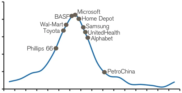
Credit Suisse — The Base Rate Book: Integrating the Past to Better Anticipate the Future (2016)
Overview unavailable.
Base Rates for Forecasting
- Introduces Credit Suisse’s The Base Rate Book, dated September 26, 2016, by Michael J. Mauboussin, Dan Callahan, and Darius Majd.
- Argues that better investment forecasts combine company-specific information—the “inside view”—with historical base rates—the “outside view.”
- Outlines research on sales growth, profitability, operating leverage, earnings growth, and cash flow returns, emphasizing persistence and regression toward the mean.
- Previews frameworks, checklists, and case studies for evaluating stocks after sharp price declines or gains.
- Includes a detailed table of contents, references to supporting data and appendices, and acknowledgments of the HOLT team’s contributions.
Base Rates Improve Forecasts
- Fundamental investing seeks gaps between the performance implied by an asset’s price and its eventual results; success depends on identifying mispriced expectations, not simply strong performers.
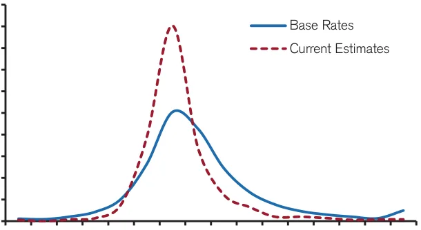
- The intuitive “inside view” builds forecasts from case-specific information and experience, but often produces excessive optimism. The “outside view” grounds expectations in outcomes from comparable cases.
- Useful reference classes must be large enough to provide robust evidence while remaining sufficiently similar to the case being evaluated; remembered individual examples are not an adequate substitute.
- The most accurate forecasts thoughtfully blend both views, giving more weight to case-specific analysis when skill dominates and to base rates when luck plays a larger role.
- Extreme outcomes tend to be followed by results closer to average. Historical data and correlations help investors estimate both the pace of this regression and the average toward which performance moves.
- The book supplies historical base rates for corporate performance and sharp stock-price moves, often using data back to 1950 that include failed or defunct companies, to improve forecasts and test others’ claims.
The goal is not to pick the winner of the race but rather the horse that has odds that are mispriced relative to its likelihood of winning.
Forecasting With Base Rates
- Intelligent investing requires understanding what current prices imply about future performance, alongside the influence of market psychology.
- The intuitive “inside view” emphasizes a situation’s unique features and extrapolates from experience, often producing overly optimistic forecasts.
- The “outside view,” or reference class forecasting, improves predictions by asking what happened in comparable situations rather than focusing solely on a particular case.
- Mergers illustrate the tension: executives emphasize strategic benefits and synergies, yet historically about 60 percent of deals have failed to create value for the acquirer.
- Useful reference classes balance sample size with relevance. Cash-funded acquisitions tend to outperform equity-funded deals, illustrating why a more specific comparison can be more informative than a broad average.
- Executives often rely on one analogy or a few memorable cases; the ideal instead is a large sample of cases similar to the decision at hand.
The outside view asks, “What happened when others were in this situation?”
Improving Forecasts with Base Rates
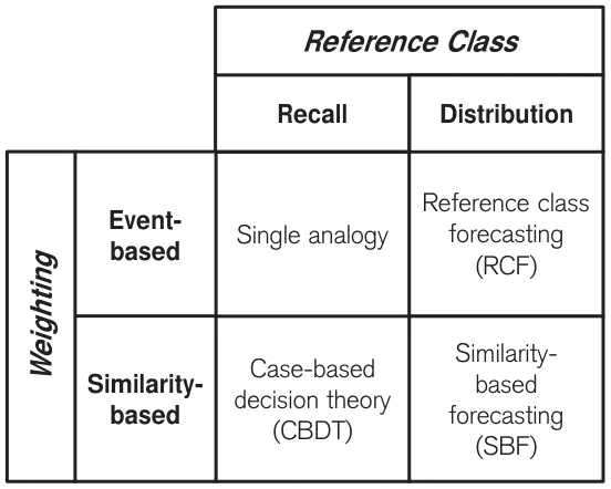
- Relying on a single analogy overemphasizes the inside view and often produces overly optimistic forecasts; recalling several comparable cases offers a broader perspective.
- Reference class forecasting uses an unbiased set of cases with equal weights, while similarity-based forecasting retains that broad set but gives greater weight to more relevant cases.
- In an experiment, private equity investors forecast returns of almost 30 percent for current deals, compared with roughly 20 percent for similar past deals; every participant expected the current deal to perform at least as well as the comparables.
- More than 80 percent of participants whose current-deal forecasts exceeded their comparable-deal returns lowered their forecasts when given the opportunity, demonstrating how an outside-view prompt can temper optimism.
- Forecasters resist the outside view because they value their own research and experience and may lack suitable reference-class data; the book addresses the data gap with base rates for corporate performance and stock returns.
Every subject wrote a rate of return for the focal project that was equal to or higher than the comparable projects.
Balancing Luck and Skill
- Kahneman and Tversky identify three ingredients of statistical prediction: base rates (the outside view), case-specific information (the inside view), and the appropriate weight for each.
- The balance between luck and skill helps determine those weights: skill-dominated activities favor case-specific evidence, while luck-dominated activities call for forecasts closer to the base rate.
- Short-term investment performance contains substantial luck, so a fund’s exceptional year is generally a reason to forecast a return closer to the peer-group average—not a repeat of its success.
- True skill can be estimated as the grand average plus a shrinkage factor times the difference between observed performance and that average. A factor of zero implies complete regression to the mean; one implies none.
- With an 8% peer average, a 12% fund return, and a 0.10 shrinkage factor, estimated true skill is only 8.4%. The correlation coefficient can serve as a practical proxy for the shrinkage factor.
Suppose you first listen to a song played by a concert pianist followed by a tune played by a novice.
Forecasting and Mean Regression
- The weight given to individual evidence versus base rates should depend on performance consistency: violinists show stable skill, whereas mutual funds’ short-term excess returns are weak indicators of skill.
- To incorporate the outside view, choose a reference class broad enough to be statistically useful but narrow enough to match the decision.
- Examine the distribution of reference-class outcomes rather than assuming a bell curve; technology IPO returns, for example, are dominated by a small fraction of companies.
- Make an informed prediction, consider a range of outcomes and probabilities, and adjust the estimate toward the average according to its reliability.
- Regression toward the mean occurs because extreme results often combine persistent skill with temporary luck. Lower correlations between successive measurements imply greater expected regression, not a guarantee that the next result will be less extreme.
You could assume that his skill of 80 would persist and that his luck, which is transitory, would be zero.
Regression's Two Illusions
- Regression toward the mean encourages two common errors: inventing causal explanations and assuming that variation declines over time. Both can mislead investors and economists.
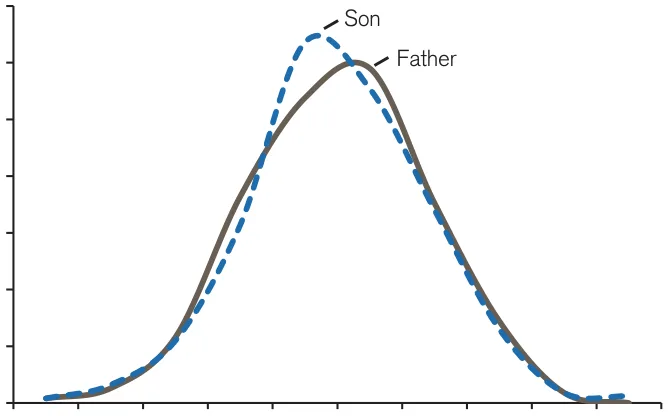
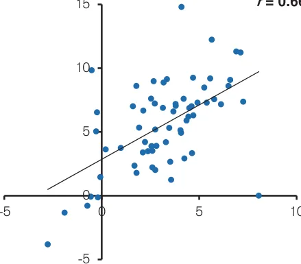
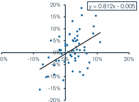
- Father–son heights illustrate regression: with a correlation of 0.50, a son's expected height lies halfway between his father's height and the population average.
- Regression also works backward: unusually tall sons tend to have fathers whose heights are less extreme. This symmetry shows why regression alone cannot establish causality.
- Extreme observations tending toward the average does not mean the overall distribution becomes more tightly clustered; individual regression and population-wide dispersion are different concepts.
- Dispersion should be checked directly using standard deviation or the coefficient of variation, which divides standard deviation by the mean. Fathers and sons have nearly identical coefficients of variation despite regression in their heights.
While it is true that tall fathers cause tall sons, it makes no sense to say that tall sons cause tall fathers.
Returns Regress Toward Average
- A study of roughly 6,600 global companies, excluding financial services and utilities, shows that high cash flow returns on investment (CFROIs) tend to decline while low returns tend to improve over a decade.
- Competition offers an intuitive explanation: high returns attract rivals, while low returns encourage disinvestment and consolidation, potentially lifting profitability.
- The same regression pattern appears when tracking returns backward in time, demonstrating that competition alone cannot explain it; imperfect correlation between periods produces regression toward the mean.
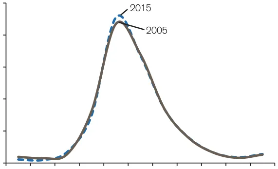
- The overall distribution of corporate returns remains nearly unchanged even as common-cause variation reshuffles individual companies within it.
- Estimating how quickly returns regress requires sector-specific correlation coefficients; stable-demand sectors such as consumer staples are expected to show greater persistence than commodity-exposed sectors such as energy.
Regression toward the mean does not rely on the arrow of time.
Sector Return Persistence
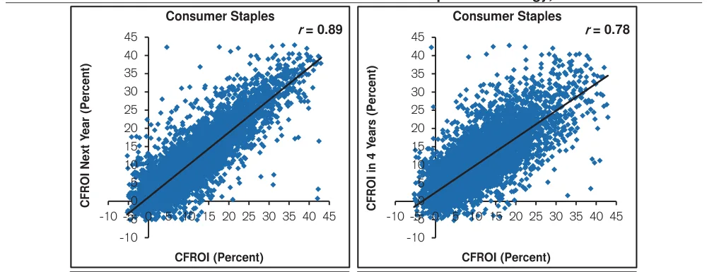
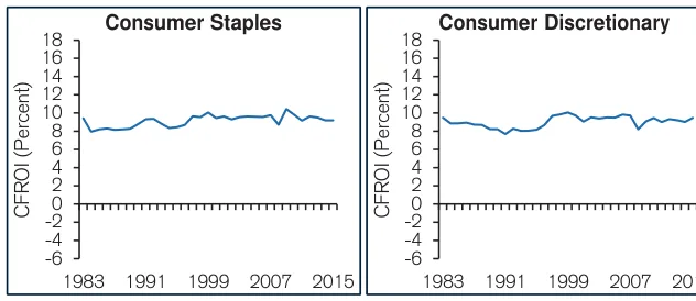
- CFROI persists much more strongly in consumer staples than in energy: correlations over one and four years are 0.89 and 0.78 for staples, versus 0.64 and 0.35 for energy.
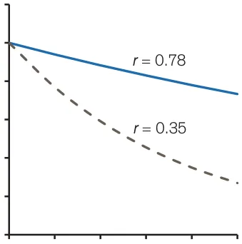
- Compounding a one-year correlation can overstate regression toward the mean. For a consumer staples company initially 10 percentage points above average, it predicts a four-year excess return of 6.3 points, compared with 7.8 points using the observed four-year correlation.
- Across ten sectors, consumer-oriented businesses generally show slower regression toward average returns, while commodity-exposed sectors tend to regress faster.
- Return persistence is also more predictable in consumer staples: its four-year correlation has a standard deviation of 0.04, compared with 0.12 for energy over 1983–2015.
- Forecasts of how excess returns fade should reflect both sector-specific persistence and its variability, rather than applying a uniform regression rate.
So using a one-year correlation coefficient overstates the rate of regression toward the mean.
Modeling Regression Toward Averages
- Sector-based regression toward the mean provides a baseline for forecasting corporate cash flow return on investment (CFROI). Using this approach, Microsoft’s CFROI would decline from 16.1% to approximately 12.6% over four years, toward the sector’s historical average of 9.0%.
- This estimate describes the average outcome for comparable companies, not a specific prediction about Microsoft’s future performance.
- Average regression conceals wide variation: some initially high-performing companies improve further, while others fall well below their sector average.
- Company-specific evidence can justify forecasts above or below the baseline, but regression toward the mean should remain a consideration in financial modeling.
- The mean itself may change over time. Historical averages are most useful for forecasting when they have been stable and the underlying environment is not expected to change substantially.
The use of a dot to capture regression toward the mean belies the richness of the underlying data.
Sector Returns and Reversion
- From 1983–2015, consumer staples averaged a 9.3% CFROI with a 0.6% standard deviation, versus 4.9% and 1.7% for energy, illustrating sharply different sector return profiles.
- Energy’s lower, more volatile returns help explain its faster regression toward the mean and lower valuation multiples relative to consumer staples.
- Percentile bands reveal differences among companies within sectors, while the coefficient of variation measures volatility relative to average returns; energy’s coefficient was 0.34 versus 0.07 for consumer staples.
- Analysts must distinguish companies reverting toward a sector average from changes in the average itself, examining drivers such as oil prices, regulation, labor costs, and depreciation.
- The text introduces corporate-performance base rates, emphasizing sales growth as the most important driver of corporate value and gross profitability—gross profit divided by assets—as a measure associated with stronger shareholder returns.
The question is whether average operating profit margins will rise, remain stable, or fall in coming years.
Growth Expectations and Base Rates
- Operating leverage measures how strongly operating profit responds to changes in sales, making sales forecast errors especially consequential for highly leveraged businesses.
- Operating profit margin underpins key valuation measures: after-tax operating profit feeds into both free cash flow and return on invested capital.
- Executives and investors prioritize earnings disclosures, while CFROI offers an inflation-adjusted measure of economic returns designed to improve comparisons across companies and over time.
- Historical studies of stocks that outperform or underperform the S&P 500 by at least 10 percent use momentum, valuation, and quality to establish subsequent return base rates, providing a starting point for less emotional investment decisions.
- Sales growth is presented as the most important driver of corporate value, yet investors and executives often overestimate growth and forecast a narrower range of outcomes than historical base rates suggest.
In some cases, knowing when to sell can be more difficult than knowing when to buy.
Forecast Biases and Base Rates
- Optimism can encourage perseverance but inflates expectations: although only about half of new businesses survive five years, over 80% of surveyed entrepreneurs put their success odds at 70% or higher.
- Overconfidence makes people more certain than their accuracy justifies and produces forecast ranges that are too narrow; CFOs’ purported 80%-confidence stock-market ranges captured actual outcomes only one-third of the time.
- Analysts’ forecasts of three-year sales growth show much less variation than historical results: their standard deviation is 8.3%, compared with 18.7% historically, suggesting substantial underestimation of uncertainty.
- Behavioral biases and incentive-driven distortions help explain why forecasts are commonly both too optimistic and too narrow.
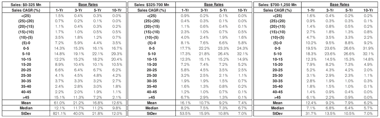
- Historical sales-growth base rates offer a benchmark for assessing forecasts. The study covers the largest 1,000 global companies since 1950, includes companies that ceased to exist, and measures inflation-adjusted growth over one, three, five, and ten years.
Forecasts are commonly too optimistic and too narrow.
Sales Growth Base Rates
- Historical sales-growth data from 1950–2015 provide reference distributions for assessing company forecasts across one-, three-, five-, and ten-year horizons.
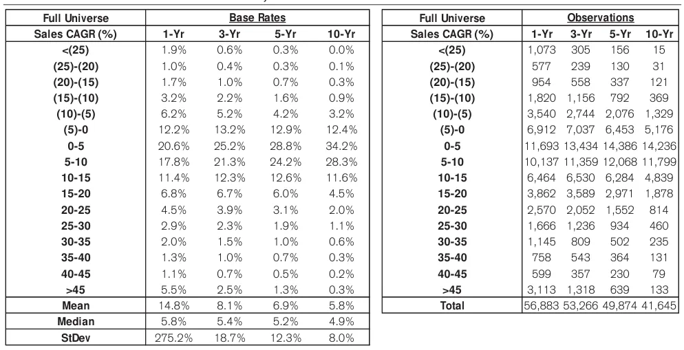
- Three-year annualized sales growth averaged 8.1%, with a median of 5.4% and a standard deviation of 18.7%. The median better represents typical outcomes because unusually high growth skews the distribution upward.
- Growth becomes less extreme over longer horizons: average annualized growth falls from 14.8% over one year to 5.8% over ten years, while the share exceeding 45% falls from 5.5% to 0.3%.
- More relevant comparisons come from grouping companies into deciles by prior-year sales, then examining the growth distribution for the appropriate size group and time horizon.
- The samples have survivorship bias because companies must survive the entire measurement period to qualify; roughly half of public companies cease to exist within ten years of listing.
- Tesla’s stated ambition to grow sales 50% annually for a decade from a roughly $6 billion base illustrates a forecast that can be assessed using historical reference classes alongside bottom-up business modeling.
About one-half of all public companies cease to exist within ten years of being listed.
Growth Forecasts Meet Reality
- The outside view tests growth forecasts against historical outcomes for companies of comparable size, making the choice of reference class essential.
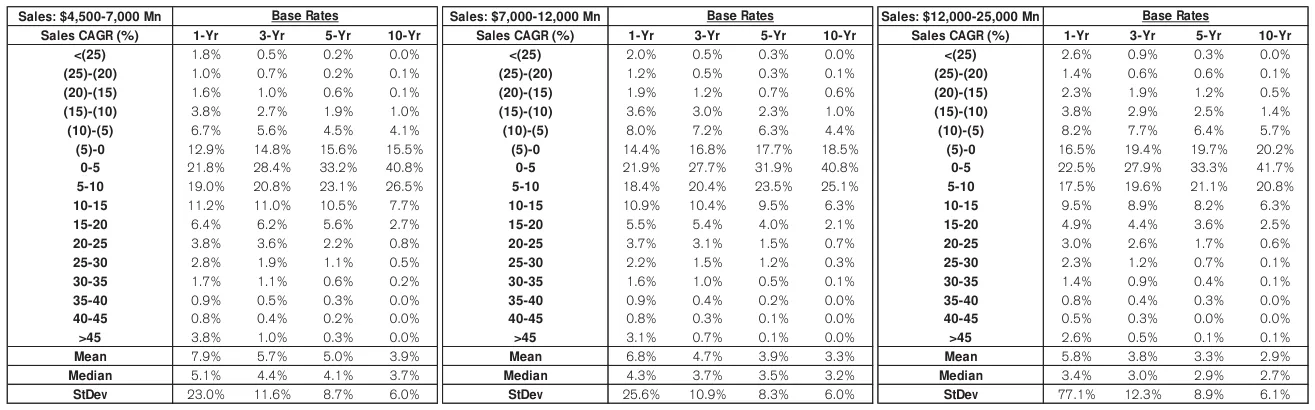
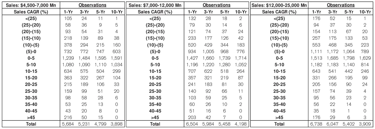
- For companies starting with $4.5–7 billion in sales, none in the historical sample sustained annual sales growth of 45 percent or more for ten years; only 0.2 percent achieved 30–35 percent growth.
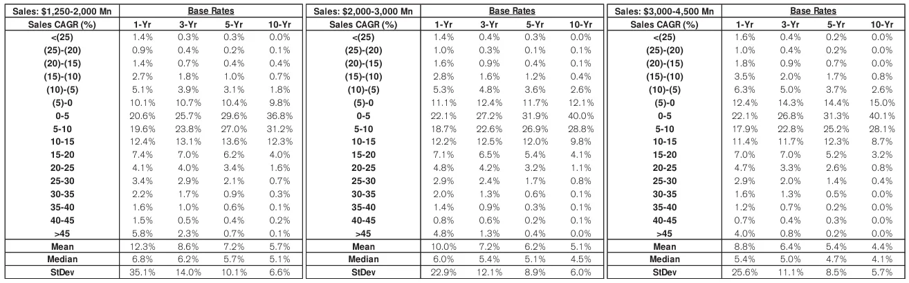
- The 1950–2015 data show that smaller companies generally grow faster: average ten-year annual sales growth falls from 12.6 percent for the smallest sales group to 5.7 percent for companies with $1.25–2 billion in sales.
- Exceptional short-term growth rarely persists over a decade. Among companies with sales below $325 million, 15.1 percent grew more than 45 percent over one year, versus 2.1 percent on a ten-year annualized basis.
- Growth outcomes become less dispersed over longer horizons, and most companies in the larger size groups shown cluster around modest long-term growth rates—supporting caution toward aggressive forecasts.
Indeed, you have to go down to 30-35 percent growth to see any companies, and even there it is only one-fifth of 1 percent of the sample.
Growth Slows With Scale
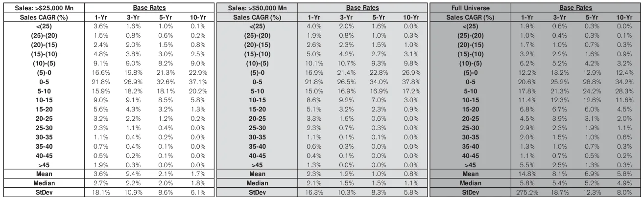
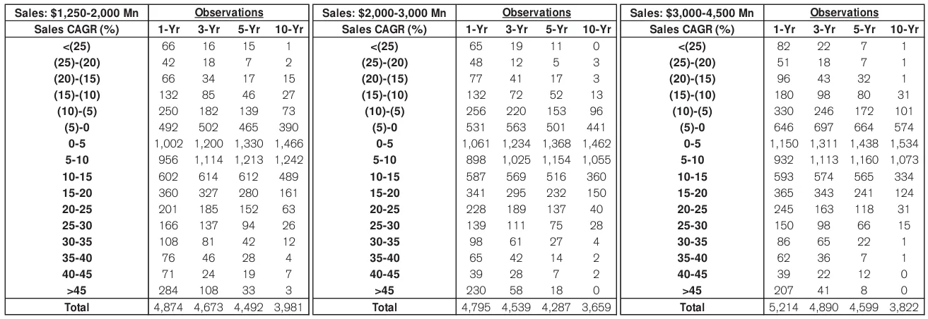
- The tables present historical sales-growth base rates by company revenue size over one-, three-, five-, and ten-year periods, providing benchmarks for evaluating growth expectations.
- Larger companies generally grow more slowly: mean ten-year annualized sales growth falls from 4.4% for companies with $3–4.5 billion in sales to 1.7% for those above $25 billion.
- Long-term growth clusters around modest rates. The 0–5% annual growth band accounts for roughly 37–42% of ten-year outcomes across the fully reported size groups.
- Growth outcomes become less dispersed over longer horizons, and extreme growth becomes rare. For companies with $3–4.5 billion in sales, growth above 45% occurs in 4.0% of one-year observations but 0.0% of ten-year observations.
- Sustained sales declines are more common among the largest companies: negative ten-year growth accounts for about 19% of outcomes in the $3–4.5 billion group, versus about 36% among companies above $25 billion.
Sales: >$25,000 Mn
Reality Checks for Growth
- The sales-growth data cover 44 reference classes defined by company size and time horizon, providing an empirical reality check for forecasts; their inflation-adjusted figures must be reconciled with forecasts that include inflation.
- As companies get larger, both average sales growth and the variability of growth decline, implying that analysts should temper growth expectations for larger firms.
- Median corporate sales growth tracks U.S. GDP growth reasonably closely, with a correlation of 0.66; real U.S. GDP grew an average of 3.2% annually from 1950 to 2015.
- Corporate sales can outgrow the domestic economy because fast-growing companies disproportionately go public, some corporate revenue growth is not captured in GDP, and overseas sales contribute to company growth.
- Sustained sales declines are common despite a natural tendency to expect growth: 23% of sampled companies shrank over three years and 20% over five years, after adjusting for inflation.
The lesson is to temper expectations about sales growth as companies get larger.
Sales Growth Base Rates
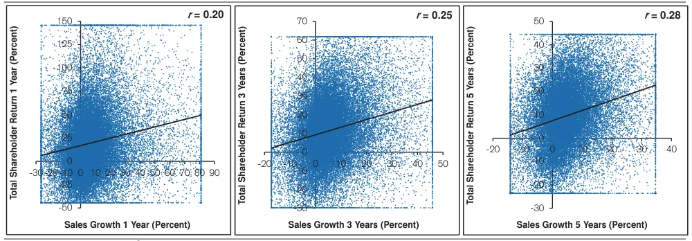
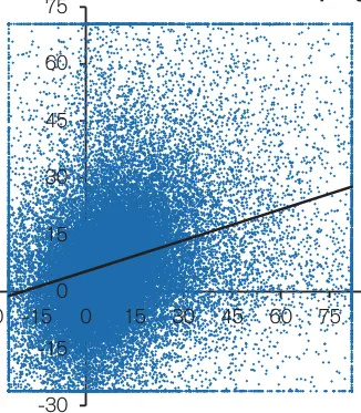
- Sales growth has only a modest positive relationship with total shareholder returns: correlations rise from 0.20 over one year to 0.28 over five years.
- Sales growth is easier to forecast than earnings growth, but accurately forecasting earnings offers a larger investment payoff, especially over longer horizons.
- Sales growth is a major driver of company value, yet its year-to-year correlation is only 0.30, indicating substantial regression toward the mean.
- For forecasts of three years or longer, the median growth rate of a relevant reference class should receive most of the weight; departures from that base rate require justification.
- Some companies will achieve exceptionally high or low growth, but forecasts near the median work best across large samples, and expectations far above it are likely to disappoint.
In fact, you might start with the base rate and seek reasons to move away from it.
Sales Growth Base Rates
- The median expected three-year sales growth rate for roughly 1,000 public companies worldwide is 1.7 percent.
- For ten companies with sales exceeding $50 billion, analysts’ inflation-adjusted three-year growth forecasts are compared with historical growth rates for similarly large companies.
- Analysts expect sales to decline at five of these ten mega companies; forecast growth rates have a standard deviation of 9.4 percent, indicating substantial variation within the group.
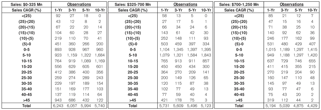
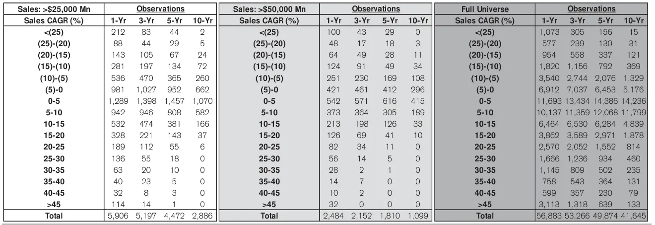
- The appendix provides historical sales-growth observation counts from 1950–2015, grouped by company sales size and measured over one-, three-, five-, and ten-year periods.
- Across the displayed size groups, longer-term growth outcomes cluster in moderate ranges, while exceptionally rapid growth becomes much rarer—highlighting the importance of matching forecasts to company size and time horizon.
Analysts expect negative sales growth for five of the ten.
Sales Growth Base Rates
- The tables report historical sales-growth distributions over 1-, 3-, 5-, and 10-year periods, grouped by company sales size and compared with the full universe.
- Annualized growth of 0–5% is the most common outcome across every displayed size group and time horizon, providing a conservative benchmark for forecasts.
- Growth outcomes become more concentrated over longer periods: roughly 63% of full-universe 10-year observations fall between 0% and 10% annualized growth.
- Sustained rapid growth is particularly rare among the largest companies. For those with sales above $50 billion, only 43 of 1,099 ten-year observations—about 4%—show annualized growth of 10% or more.
- Declining sales remain a meaningful long-term possibility: 7,041 of 41,645 full-universe ten-year observations, approximately 17%, show negative growth.
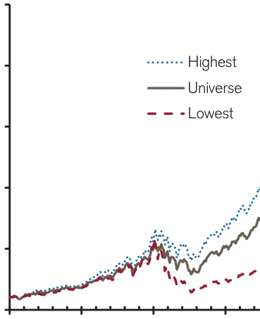
Total Return for the Highest and Lowest Quintiles of Profitability (1990-January 2016)
Gross Profitability and Returns
- Benjamin Graham’s late-career stock screen combined valuation and quality criteria, seeking companies that were both cheap and high quality.
- Gross profitability—revenue minus cost of goods sold, divided by total assets—provides a measure of business quality that is not positively correlated with traditional value measures.
- Research finds that gross profitability persists over time and that highly profitable companies deliver stronger shareholder returns despite starting at higher price-to-book ratios.
- Profitability helps explain stock returns across international markets and has become a factor in prominent asset-pricing models, including Fama and French’s model.
- Gross profitability can give a different investment signal from price-to-earnings ratios; Amazon’s roughly 540 trailing P/E at year-end 2015 illustrates how expensive a stock can appear through an earnings-based lens alone.
Because it was toward the end of Graham’s life, some refer to the list as Graham’s “last will.”
Gross Profitability Persists
- Amazon’s 2015 gross profitability—gross profit divided by total assets—was 0.54, comfortably above Novy-Marx’s attractive threshold of 0.33, which Amazon had exceeded for most of its history.
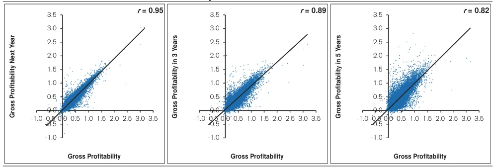
- Gross profitability is highly persistent: correlations with future profitability are 0.95 after one year, 0.89 after three years, and 0.82 after five years.
- The persistence analysis covers more than 40,000 company-years among the world’s largest firms from 1950–2015, including failed companies but excluding financial services and utilities.
- Profitability quintiles show little regression toward the mean, with the highest-to-lowest spread narrowing only from 0.54 to 0.49; last year’s profitability is therefore a sensible starting point for forecasts.
- Gross profitability’s simple correlation with shareholder returns is weak, though stronger over longer horizons: 0.06 over one year versus 0.24 over five years. The cited researchers do not recommend relying on this simple correlation.
Given this stability, a sensible forecast is to start with last year’s profitability and seek reasons to move away from it.
Profitability Persistence by Sector
- Ranking stocks into gross-profitability quintiles offers a way to construct and compare portfolios; the analysis tracks the largest 1,000 U.S. industrial and service companies from 1990 through January 2016, with monthly rebalancing.
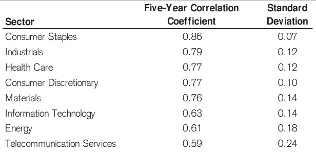
- Sector-specific base rates make profitability forecasts more relevant by identifying both the appropriate mean and the expected speed of regression toward it; the analysis covers eight sectors, excluding financial services and utilities.
- Gross profitability is more persistent in consumer discretionary companies than in energy companies: five-year correlations are 0.77 and 0.61, respectively, implying slower mean reversion in consumer discretionary.
- Consumer-oriented sectors generally exhibit slower profitability mean reversion, while sectors exposed to technology or commodities tend to revert more rapidly.
- Persistence also varies over time: correlation standard deviations are 0.10 for consumer discretionary and 0.18 for energy, indicating greater uncertainty around energy's profitability persistence.
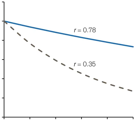
A high r suggests slow regression, and a low r means more rapid regression.
Profitability and Operating Leverage
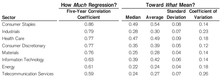
- More than 60 years of sector data provide benchmarks for how quickly gross profitability regresses toward the mean and which mean to use; this population-level tendency does not necessarily apply to individual companies.
- Profitability persistence varies by sector: five-year correlations range from 0.86 for consumer staples to 0.59 for telecommunications, indicating different rates of regression.
- Sector profitability distributions are often nonnormal, making medians useful alongside averages. Consumer discretionary has higher average profitability and lower relative variability than energy.
- Operating leverage helps connect changes in sales, costs, and operating margins to earnings, making it important for anticipating revisions to market expectations.
- Investors can earn meaningful excess returns by correctly anticipating earnings that differ substantially from expectations, but analysts often overestimate growth—especially when high-operating-leverage companies report weak sales. Buy-side analysts are generally more optimistic and less accurate than sell-side analysts.
Analysts are commonly too optimistic about earnings growth and often miss estimates by a wide margin.
Operating Leverage and Earnings
- Operating leverage measures how strongly operating profit, or earnings before interest and taxes (EBIT), responds to changes in sales.
- Analyzing sales volume, price and mix, economies of scale, and cost efficiencies helps explain earnings changes and anticipate revisions to market expectations; financial leverage further affects earnings variability.
- Sales growth does not translate uniformly into profit growth: a company’s cost structure determines how much additional revenue reaches operating profit.
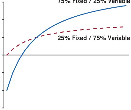
- High fixed costs amplify both gains and losses as sales change, while variable costs move with output and limit operating leverage. Theme parks illustrate high operating leverage, with roughly three-quarters of costs fixed.
- In the illustration, both businesses earn a 20% operating margin at $10 million in sales. At $25 million, the high-fixed-cost business approaches 60% versus just over 30% for its counterpart; at $5 million, it falls to a −40% margin while its counterpart breaks even.
If sales shrink, fixed costs don’t budge and profits fall sharply. Conversely, profits rise substantially if sales grow.
Leverage and Sales Growth
- A higher ratio of fixed assets to total assets is associated with higher fixed costs and greater operating leverage, making operating profits more sensitive to changes in sales.
- All costs are variable in the long run: companies can cut costs when sales decline, while industry growth gradually dilutes incumbents’ advantages from high fixed costs.
- Data for the largest 1,000 global companies, excluding financial services and utilities, show that operating leverage is especially pronounced during recessions and subsequent recoveries.
- Debt adds interest expense and financial leverage, amplifying earnings fluctuations; companies with both high operating and financial leverage therefore face greater earnings risk.
- Economic growth provides a starting point for sales forecasts, but sensitivity varies by sector: consumer discretionary and industrial sales correlate more strongly with U.S. GDP growth than consumer staples and health care sales.
It is important to underscore that all costs are variable in the long run.
Drivers of Sales Growth
- Sales growth’s relationship with U.S. GDP varies substantially by sector: consumer discretionary and industrials show strong correlations, while energy shows a very weak correlation.
- Industry growth is analysts’ primary consideration in sales forecasts, but forecasts must account for industry life cycles: rapid expansion typically gives way to slower growth along an S-curve.
- Extrapolating rapid growth can lead to severe overcapacity. Color television manufacturers built capacity for 14 million units in the late 1960s, although unit sales peaked at 6 million.
- Mergers and acquisitions accounted for about one-third of large companies’ sales growth in one study, but large deals can alter operating leverage and substantial value creation is difficult.
- Market shares tend to fluctuate in emerging industries and stabilize as industries mature. Although market share correlates positively with profitability, competitor-focused objectives such as market share targets can harm profitability.
But they extrapolated the sharp growth and failed to recognize the top of the S-curve.
Growth, Margins, and Value
- Sales growth creates value only when returns on investment exceed the cost of capital; companies can increase profits while destroying economic value.
- The threshold margin is the operating profit margin needed to earn the cost of capital. More capital-intensive companies require higher margins to break even economically.
- Understanding changes in operating margins requires separating the effects of sales volume, pricing, product mix, operating leverage, and economies of scale.
- Pricing power can improve margins when price increases exceed incremental costs, but demand sensitivity matters: a study of roughly 370 goods found that a 1% price change produced an average 1.76% change in demand.
- A shift toward higher-margin products can outweigh falling sales: from 2011 to 2015, Goodyear’s sales fell 28% and unit volume fell 8%, yet operating income rose nearly 50% as it shifted toward premium tires.
Indeed, sales growth destroys value for a company earning a return below the cost of capital.
Understanding Operating Leverage
- Businesses incur preproduction costs before generating revenue, but accounting treatment differs: physical facilities are typically capitalized and depreciated, while research and software development investments are mostly expensed.
- Operating leverage arises when growing sales spread preproduction costs over more units, lifting profit margins with relatively little incremental investment.
- Capacity utilization helps assess operating leverage: operating margins generally expand as utilization rises and contract as it falls.
- Economies of scale differ from operating leverage because they reduce the cost of performing activities per unit as volume grows; confusing the two can lead to overly optimistic assumptions about future costs.
- Home Depot illustrates economies of scale: its gross margin rose from 27.7% to 29.9% between fiscal 1996 and 2001 as greater purchasing power helped secure better supplier prices.
- Cost efficiencies can also improve margins through cheaper execution or redesigned activities, but these improvements are independent of sales changes and should be distinguished from operating leverage.
Mistaking operating leverage for economies of scale may lead to the incorrect conclusion that unit costs will decline even as the company expands to meet new demand.
Operating Leverage Across Sectors
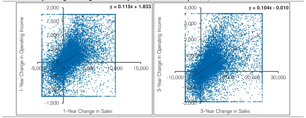
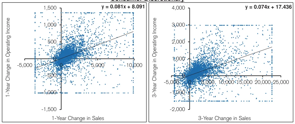
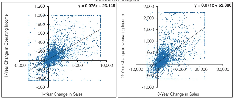
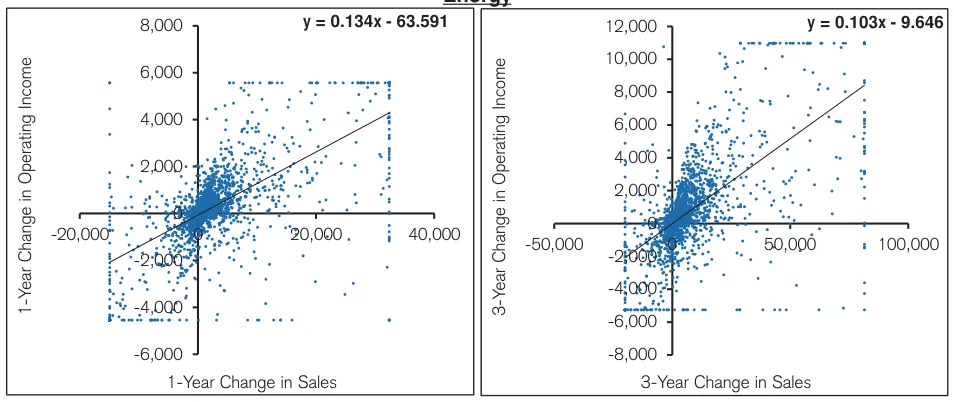
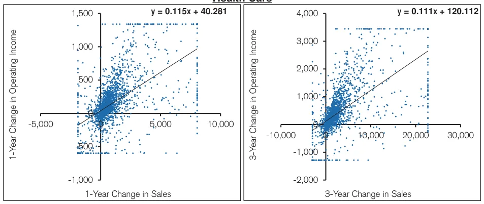
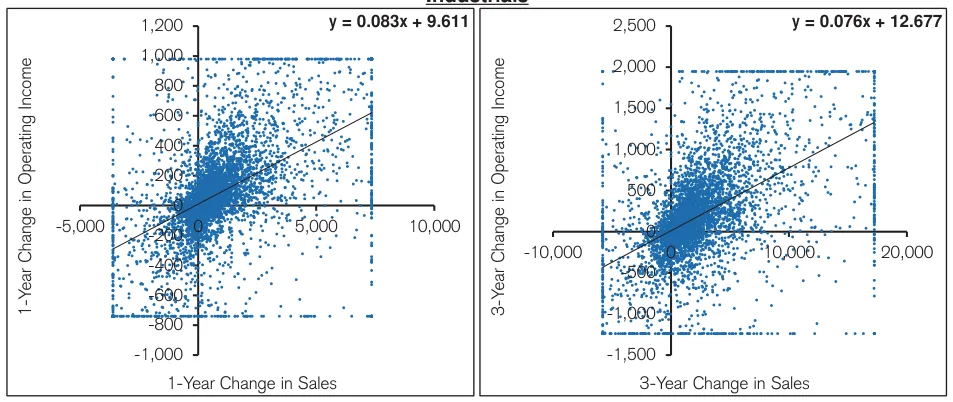
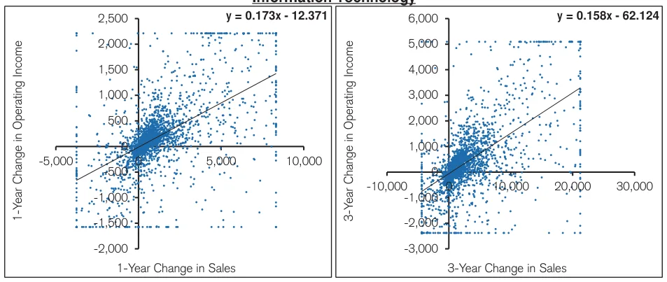
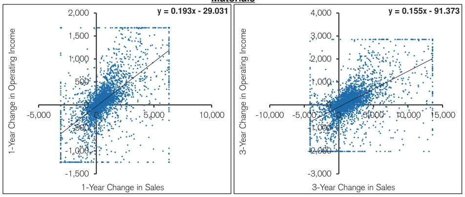
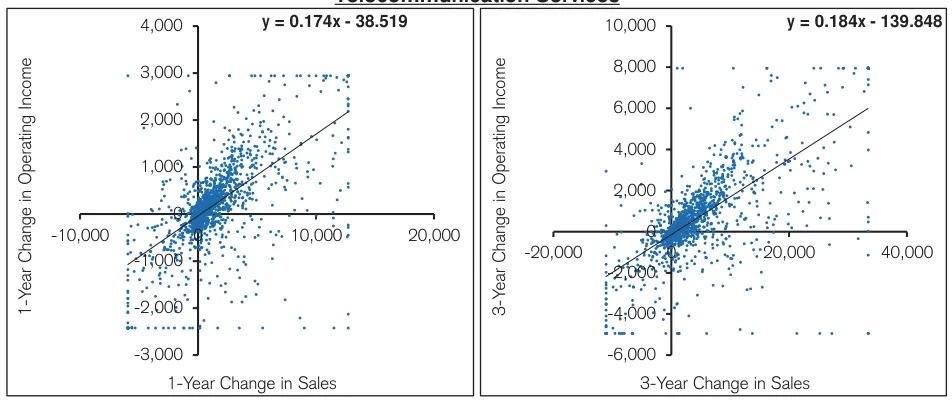
- The study estimates operating leverage using the regression slope between changes in sales and operating profit, calling this measure the “operating margin beta.”
- Data cover the top 1,000 global companies by market capitalization from 1950–2015, excluding financial services and utilities, with results measured over one- and three-year periods.
- The overall beta is approximately 0.11: a $1 change in sales is associated with roughly an $0.11 change in operating profit.
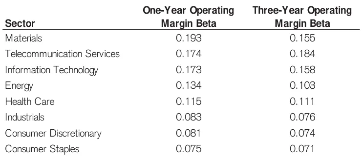
- Sector differences are substantial: materials has the highest one-year beta (0.193), while telecommunications has the highest three-year beta (0.184). Consumer staples has the lowest beta over both horizons (0.075 and 0.071).
- Three-year betas are lower than one-year betas in seven of eight sectors; telecommunications is the exception. These differences show why sector-specific benchmarks matter when estimating profit sensitivity to sales.
The way to interpret the β is that for every $1.00 change in sales, operating profit changes by approximately $0.11.
Leverage and Earnings Volatility
- Analyst forecast errors tend to be larger in industries with high operating margin beta, making a thorough assessment of operating leverage especially important.
- Forecast accuracy depends on economic conditions: analysts’ usual optimism serves them better when industrial production accelerates, but leads to substantial misses when conditions deteriorate.
- Analysts outperform management in forecasting earnings for businesses with high operating margin beta, while management does better when firms face unusual issues such as losses, inventory increases, or excess capacity.
- Management forecasts beat analyst forecasts only about half the time overall, suggesting that executives’ information advantage may matter less than macroeconomic factors.
- Operating-income volatility determines a company’s asset beta independently of financing choices; financial leverage then amplifies earnings volatility because interest expense acts as an additional fixed cost.
Analysts, who are normally optimistic, are rewarded when economic conditions are favorable and miss the mark substantially when conditions are poor.
Leverage and Earnings Volatility
- Debt amplifies earnings volatility because fixed interest payments magnify fluctuations in operating profit; in the example, indebted Company B’s pretax profit ranges from $50 to $90.
- Debt-to-total-capital ratios can misrepresent financial risk when companies hold substantial cash. Apple’s roughly 14 percent ratio in June 2016 coexisted with a net cash position exceeding $100 billion, even after potential repatriation taxes.
- Higher credit ratings generally accompany stronger operating margins, lower debt levels, greater interest coverage, and lower default rates.
- Companies with high operating leverage tend to use less financial leverage, choosing conservative capital structures to limit overall earnings volatility.
- U.S. corporate cash-to-assets ratios rose from 7 percent in 1980 to about 16 percent at the time of writing. The text links this partly to R&D-intensive businesses using cash buffers to offset the risks of fixed or quasi-fixed research costs.
The highest profit ($90) is 80 percent greater than the lowest profit ($50). The addition of debt creates more volatility in earnings and may suggest different values for the businesses.
Growth and Value Creation
- Sales and profit growth do not automatically create shareholder value; incremental investments must earn more than the cost of capital.
- The incremental threshold margin is the operating margin required on new sales to earn the cost of capital. Greater fixed-capital and working-capital requirements raise this hurdle.
- The incremental threshold margin equals the combined incremental fixed- and working-capital rates multiplied by the cost of capital, divided by [(1 + cost of capital) × (1 − tax rate)].
- In the example, a company growing sales by 8% with a 10% cost of capital needs an incremental operating margin of approximately 8.4%. Achieving that margin makes its growth value neutral rather than value creating.
- The overall threshold margin combines prior-year operating income with the required profit on incremental sales, then divides by total current sales, linking growth and profitability to shareholder value.
This demonstrates that growth does not equal value creation.
Operating Margins and Value
- A company creates value by earning more than its capital’s opportunity cost; operating profit margin, defined as operating income divided by sales, is a key profitability indicator.
- Subtracting cash taxes from operating profit yields net operating profit after tax (NOPAT). NOPAT underpins both free cash flow, after subtracting investments, and return on invested capital (ROIC).
- ROIC combines profitability with capital velocity. Cost leaders such as Wal-Mart typically pair low margins with high sales relative to invested capital, while differentiated businesses such as Tiffany tend toward high margins and lower capital velocity.
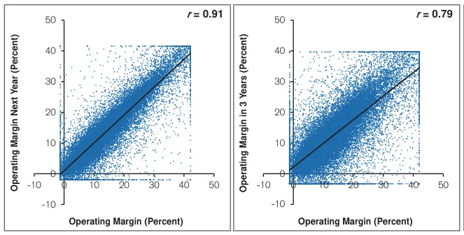
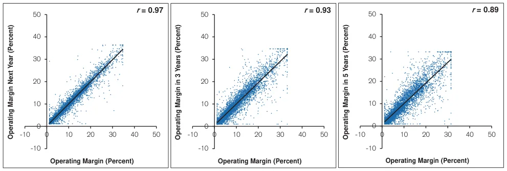
- Operating margins are highly persistent: correlations between current margins and margins one, three, and five years later are 0.91, 0.79, and 0.72, respectively, making current profitability informative about future performance.
- The evidence covers more than 40,000 company-years among the world’s top 1,000 firms by market capitalization from 1950–2015, including failed firms but excluding financials and utilities. Historical comparisons also reflect changes in accounting rules, notably stock-based compensation expensing around 2005.
FCF is the cash that is distributable to a company’s debtors and equity holders, and hence is the lifeblood of corporate value.
Operating Margin Persistence
- Operating profit margins show limited regression toward the mean: over ten years, the gap between the highest and lowest margin quintiles narrows only from 0.21 to 0.15.
- Last year’s operating margin is therefore a sensible forecasting baseline; departures from it should be supported by specific reasons.
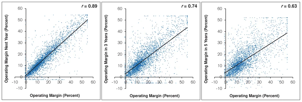
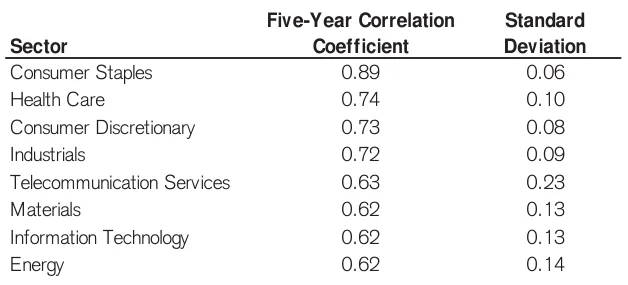
- Sector-level analysis offers more relevant base rates, although it reduces sample size. Consumer staples margins are more persistent than energy margins, with five-year correlations of 0.89 versus 0.63.
- Consumer-oriented sectors generally exhibit slower regression toward the mean than sectors more exposed to commodities or technology, making sector-specific assumptions important.
- The persistence of margins is itself more stable in consumer staples: its historical correlation standard deviation is 0.06, compared with 0.14 for energy, indicating greater uncertainty in energy-sector forecasts.
Given this stability, a sensible approach is to start with last year’s operating margin and seek reasons to move away from it.
Uneven Profit Margin Gains
- Operating profit margins regress toward sector-specific averages, but this pattern applies to populations rather than necessarily to every individual company.
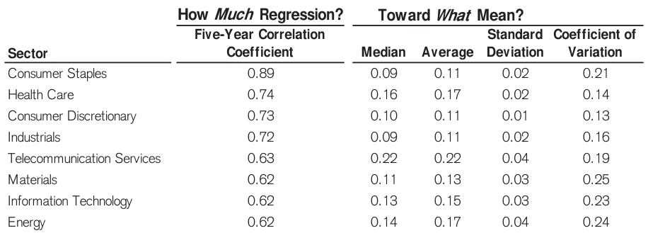
- Five-year margin correlations vary substantially across sectors: consumer staples show the greatest persistence at 0.89, compared with 0.62 for materials, information technology, and energy.
- Sector averages and variability provide useful forecasting benchmarks; average margins range from 11% to 22%, while energy margins are more volatile than consumer staples margins.
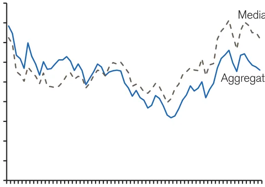
- Among the top 1,000 companies, excluding financial services and utilities, aggregate and median operating margins have risen since the mid-1980s as the economy shifted toward higher-margin service and knowledge businesses.
- Margin expansion has been concentrated in the highest-margin companies: the top quintile rose from 21% in 1985 to 31% in 2015, while the bottom three quintiles remained roughly flat over the full period. Because quintiles are reconstituted annually, these results do not track a fixed set of companies.
But the top two quintiles, and especially the highest one, show substantial expansion. For example, the operating profit margin for the highest quintile went from 21 percent in 1985 to 31 percent in 2015.
Margins and Market Composition
- Operating profit margins rose for the top-performing 20% of companies over 1950–2015, highlighting gains concentrated among the strongest earners.
- The sector composition of the largest 1,500 U.S. companies changed substantially: energy, materials, and industrials fell from 50% of market capitalization in 1980 to 19% in 2015, while healthcare and technology rose from 18% to 34%.
- Historical average margins differ sharply by sector: telecommunications averaged 21.0%, healthcare 15.7%, and information technology 14.5%, compared with roughly 8% for consumer sectors and industrials.
- Margin stability also varies: consumer staples had a standard deviation of just 1.0 percentage point, versus 5.3 for telecommunications and 4.0 for information technology.
- The exhibits present both sector-level trends and quintile breakdowns, underscoring the need to consider industry mix and within-sector differences when assessing profitability.
Over the same period, the healthcare and technology sectors went from 18 to 34 percent of the market capitalization.
Earnings and Their Limits
- Executives and investors regard earnings as a leading measure of corporate performance, underpinning widespread earnings guidance and the popularity of price-earnings valuation multiples.
- Earnings can rise without creating shareholder value because accounting choices affect reported results, while earnings omit businesses’ capital requirements and cost of capital.
- Research shows that earnings announcements convey information to markets, increasing trading volume and stock-price volatility; international accounting standards have also strengthened their information content outside the United States.
- Evidence on earnings’ evolving relevance is mixed: some research finds increased information content since 2001, while other studies suggest intangible investment has reduced their usefulness. Each quarterly announcement reflects only an estimated 1–2 percent of the total new information available annually.
- More detailed earnings disclosures and guidance help analysts revise forecasts faster and more frequently, with less disagreement. Yet roughly 40 percent of large U.S. companies provide no earnings guidance, and fewer than a quarter forecast revenue, expenses, and earnings together.
As a result, it is possible to increase earnings without creating value.
Earnings Expectations and Overconfidence
- The gap between adjusted “Street” earnings and GAAP earnings has widened as companies exclude more special or non-cash items. Whether this primarily improves forecasting or boosts perceived value is unclear, but Street EPS correlate more closely with stock price movements.
- EPS growth creates shareholder value when it comes from investments earning more than the cost of capital. Investors who correctly anticipate earnings that differ substantially from current forecasts can earn substantial excess returns.
- Earnings growth rates have limited persistence, making past growth a weak predictor of future growth. Examining accrual reliability can improve forecasts because less reliable accruals are associated with less persistent earnings.
- Analysts’ earnings growth forecasts tend to be both too optimistic and too narrow, particularly for growth companies and hard-to-value firms during bullish periods. Forecast growth rates have a standard deviation of 19.2%, compared with 34.6% for historical outcomes.
- Investors should focus on gaps between expectations embedded in stock prices and likely business performance. Success requires judging whether expectations are too high or low, rather than forecasting earnings with pinpoint accuracy.
Forecasts are commonly too optimistic and too narrow.
Earnings Growth Base Rates
- Sales are the main driver of corporate value, but earnings are the standard measure for communicating results; sales growth is more persistent than earnings growth yet less predictive of shareholder returns.
- The study examines net income growth among the top 1,000 global companies by market capitalization from 1950–2015, including companies that subsequently died, and adjusts figures for inflation.
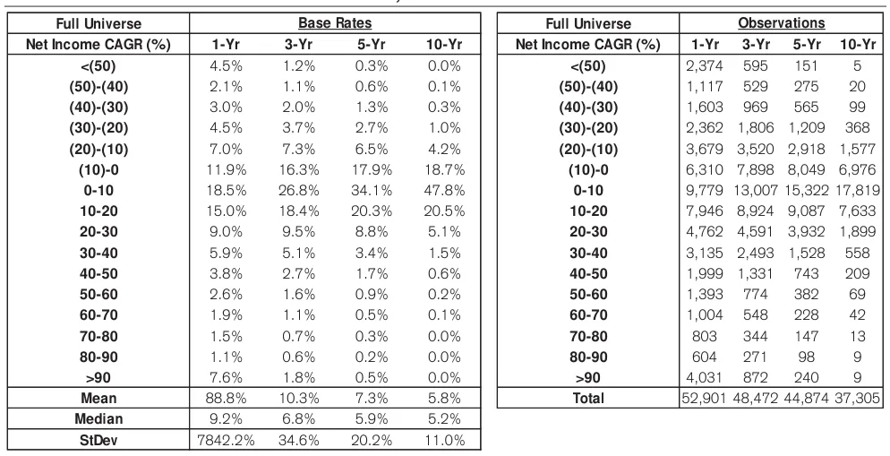
- Five-year annualized net income growth averaged 7.3%, with a median of 5.9% and a standard deviation of 20.2%; the right-skewed distribution makes the median a better measure of typical growth.
- Growth outcomes become less extreme over longer periods: 47.8% of ten-year observations show annualized growth of 0–10%, compared with 18.5% of one-year observations.
- To make historical base rates more relevant for forecasting, the analysis next groups companies into deciles by starting annual sales and examines growth distributions within each size group.
Sales are the most important driver of corporate value, while earnings are the most common metric to communicate results and to establish value.
Benchmarking Earnings Growth
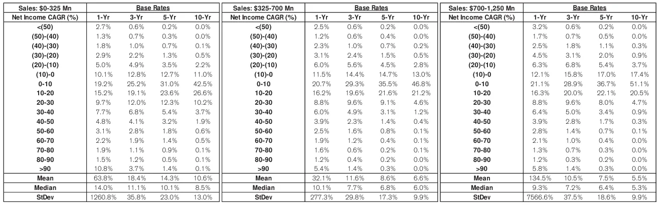
- Historical net income growth data from 1950–2015 provide reference classes based on company sales, helping analysts assess forecasts against comparable firms.
- The framework covers 44 reference classes: 11 sales-size groups, including companies with sales above $50 billion, across one-, three-, five-, and ten-year horizons.
- Alphabet’s projected inflation-adjusted earnings growth of roughly 15% annually over three years falls into a range achieved by only 15.4% of companies in its mega-company reference class.
- The displayed tables show growth outcomes becoming less dispersed over longer horizons, with extreme gains and losses increasingly rare and modest positive growth more common.
- Large gaps between short-term means and medians reveal the influence of extreme outcomes, underscoring why full distributions offer a better reality check than averages alone.
Going out to the column under “3-Yr,” we see that 15.4 percent of companies achieved this feat.
Earnings Growth Base Rates
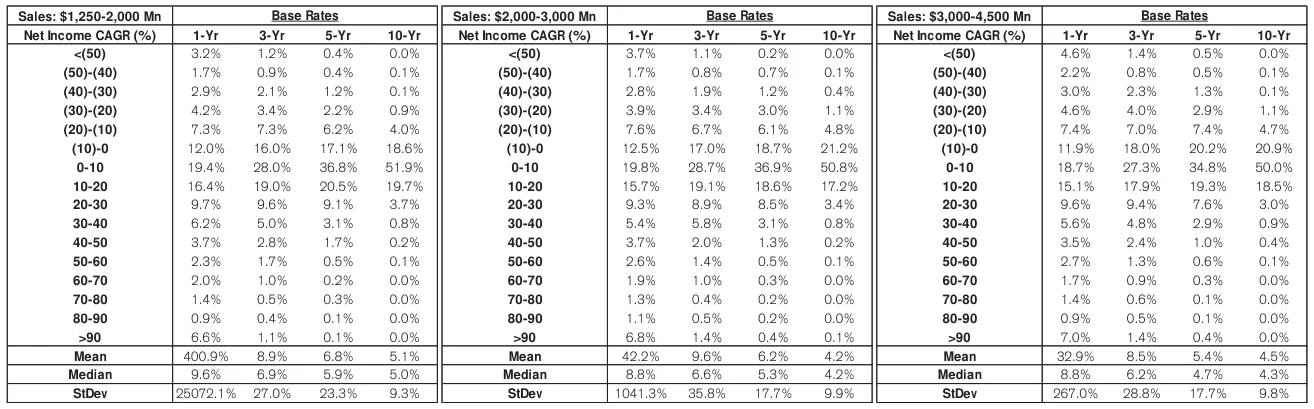
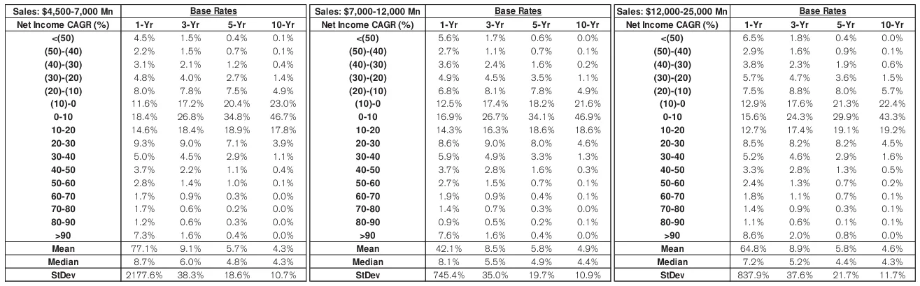
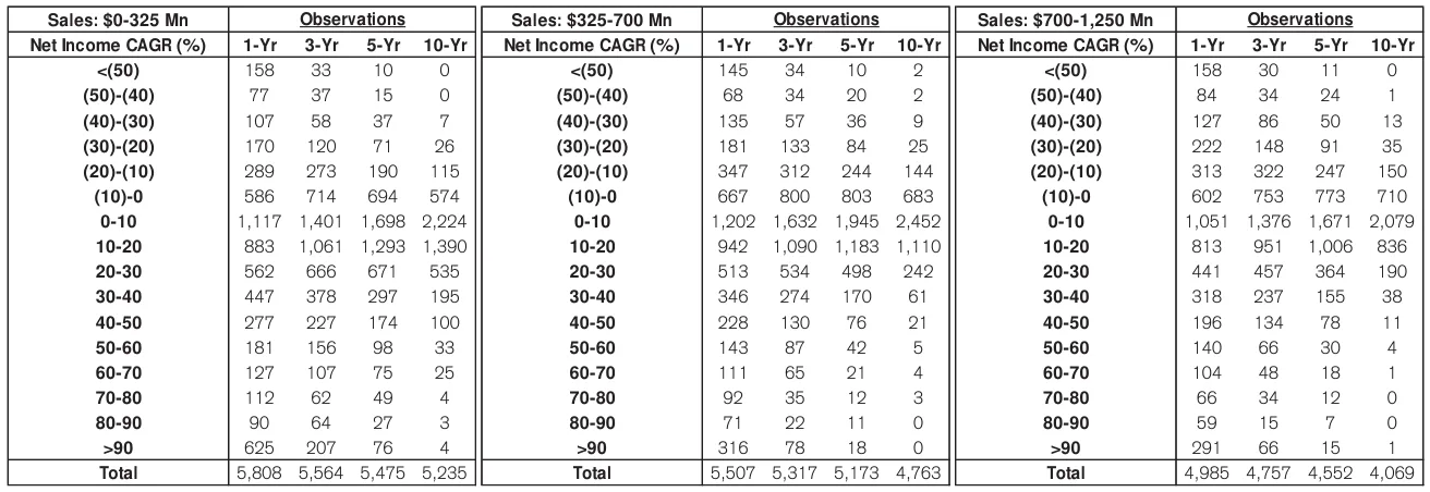
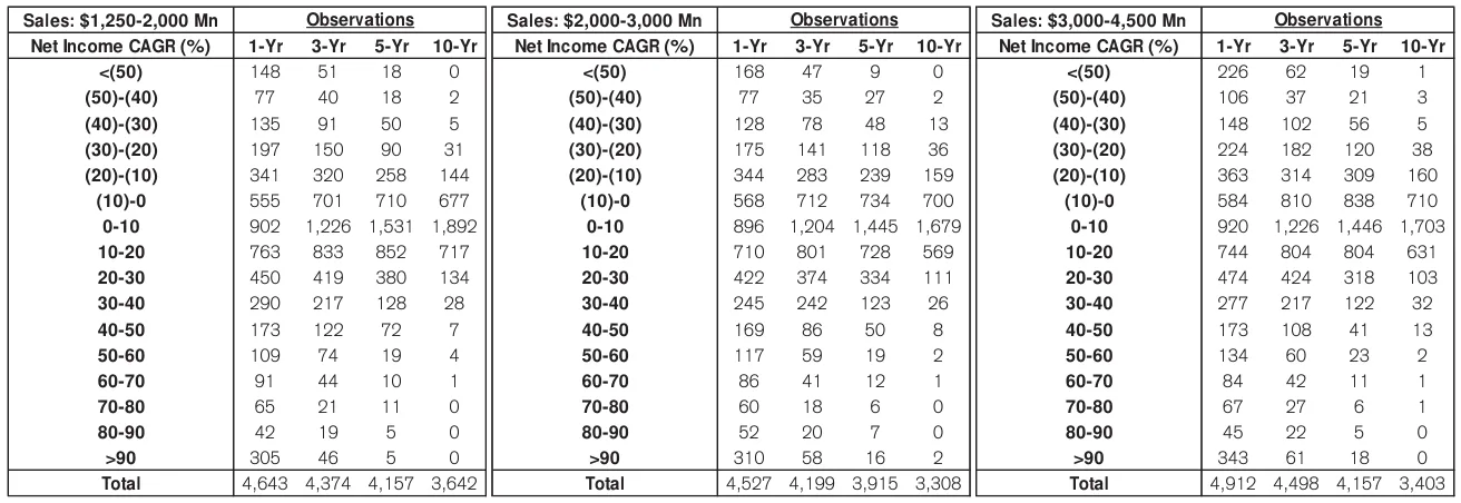
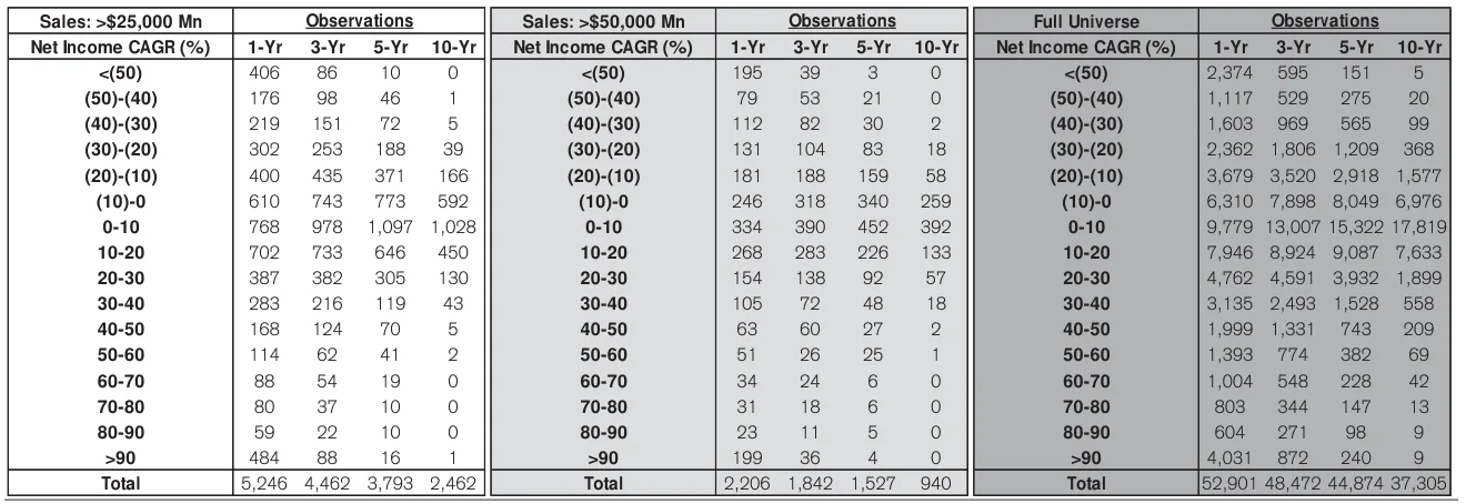
- The tables report distributions of net income compound annual growth rates over one, three, five, and ten years, grouped by company sales, with fully displayed sales bands ranging from $2 billion to $12 billion.
- Growth outcomes become more concentrated over longer horizons: roughly 47–51% of companies in the fully displayed sales bands record ten-year annualized earnings growth of 0–10%, compared with about 17–20% over one year.
- Extreme short-term gains rarely persist: approximately 7% of companies in these bands show one-year earnings growth above 90%, but only 0–0.1% achieve that annualized rate over ten years.
- One-year averages can be heavily distorted by extreme outcomes. For companies with $4.5–7 billion in sales, mean growth is 77.1%, versus a median of 8.7%; their ten-year mean and median both equal 4.3%.
- Long-term earnings declines remain meaningful: roughly 21–23% of companies in the fully displayed sales bands have ten-year annualized growth between −10% and 0%, cautioning against assuming that earnings inevitably increase.
Mean 77.1%
Size Tempers Earnings Growth
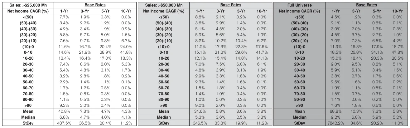
- Historical net income growth distributions show that larger companies generally have lower median growth rates and less variability, making company size an important forecasting reference.
- Across the full universe, median annualized net income growth declines from 9.2% over one year to 5.2% over ten years; the ten-year mean is 5.8%.
- For companies with sales above $50 billion, median annualized growth is just 3.3% over ten years, compared with 4.1% for companies above $25 billion.
- Long-term outcomes cluster around modest growth: 47.8% of the full universe records ten-year annualized growth between 0% and 10%, while growth above 40% is rare.
- Extreme one-year outcomes sharply inflate average growth and volatility, so medians and longer-term distributions offer a more grounded perspective than short-term averages alone.
Exhibit 6 reveals that the variance in net income growth rates for ten years declines with size, underscoring that it is sensible to temper expectations about net income growth for large companies.
The Perils of Growth Promises
- U.S. corporate profit growth and GDP growth were moderately correlated from 1947 to 2015. Both averaged 3.2% annually after inflation, but profits were far more volatile.
- Warren Buffett warns that public promises of sustained rapid earnings growth are deceptive and dangerous because very few large companies can deliver them over decades.
- A test of the 200 highest-earning companies in 1990 supports Buffett’s warning: only 14 of the 162 surviving companies achieved at least 15% annual net income growth during 1990–1999, and none of those 14 exceeded 15% in the following decade.
- Buffett distinguishes reasonable internal goals and cautiously expressed hopes from firm public growth forecasts that create pressure to meet unrealistic targets.
- Lofty earnings promises can distort executive behavior, encouraging economically unsound decisions and accounting manipulation that may escalate from fudging into fraud.
These can turn fudging into fraud. (More money, it has been noted, has been stolen with the point of a pen than at the point of a gun.)
Earnings Growth Base Rates
- Investors should be skeptical of CEOs’ ambitious forecasts: genuine foresight is difficult to distinguish from excessive optimism or deception.
- Inflation-adjusted earnings declines are common: 33% of sampled companies experienced negative growth over one year, and 24% over ten years.
- Net income growth correlates positively with total shareholder returns, with correlations rising from 0.20 over one year to 0.40 over five years, making accurate forecasts valuable but difficult.
- Earnings growth shows almost no year-to-year persistence: a correlation of -0.05 suggests unusually strong or weak growth tends to revert toward the average, with a slight tendency to overshoot it.
- For forecasts covering three years or longer, the relevant reference class’s median earnings growth should receive most of the weight; investors should start with this base rate and require reasons to depart from it.
A few of these managers will prove prophetic — but others will turn out to be congenital optimists, or even charlatans.
Earnings Growth Base Rates
- Net income growth shows little persistence: correlations are −0.05 over one-year horizons, −0.23 over three years, and −0.24 over five years, suggesting a tendency toward reversal rather than sustained momentum.
- Analysts expect median three-year net income growth of 7% for the world's largest 1,000 public companies, which the text describes as roughly consistent with GDP growth of 2–3%.
- Forecast inflation-adjusted earnings growth for ten companies with sales above $50 billion is compared with historical growth distributions for similarly large companies, providing a base-rate benchmark for expectations.
- The appendix tabulates historical net income growth observations from 1950–2015 by company sales bracket and by one-, three-, five-, and ten-year horizons.
- Across the fully displayed sales brackets, longer-horizon growth concentrates increasingly in the 0–10% annual range, while extreme gains and losses become much less common—highlighting the difficulty of sustaining exceptional growth.
The median expected growth rate is seven percent, which is roughly consistent with GDP growth of two to three percent.
Earnings Growth Base Rates
- The tables report historical net income compound annual growth rates over 1-, 3-, 5-, and 10-year periods, grouped by company sales, using Credit Suisse HOLT data.
- Across every fully shown sales group, 0–10% annual earnings growth is the most common outcome at each time horizon, providing a baseline for evaluating forecasts.
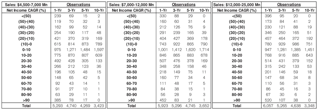
- Extreme growth outcomes become much rarer over longer periods. Among companies with sales above $25 billion, growth exceeding 90% appears in 484 one-year observations but only one ten-year observation.
- Long-term earnings declines remain meaningful: companies with sales of $7–12 billion have 790 ten-year observations of growth between −10% and 0%, compared with 1,714 between 0% and 10%.
- The number of observations falls as the measurement horizon lengthens. For companies with sales above $50 billion, the sample drops from 2,206 one-year observations to 940 ten-year observations, so comparisons involve different-sized samples.
The Base Rate Book
CFROI and Return Persistence
- Cash Flow Return on Investment (CFROI) measures economic returns using inflation-adjusted cash flows and operating assets, enabling comparisons across companies, industries, geographies, and time.
- CFROI helps investors identify value-creating companies and assess the expectations embedded in share prices.
- The calculation accounts for the finite economic lives of depreciating assets and the residual values of non-depreciating assets; financial companies are better assessed using Cash Flow Return on Equity (CFROE).
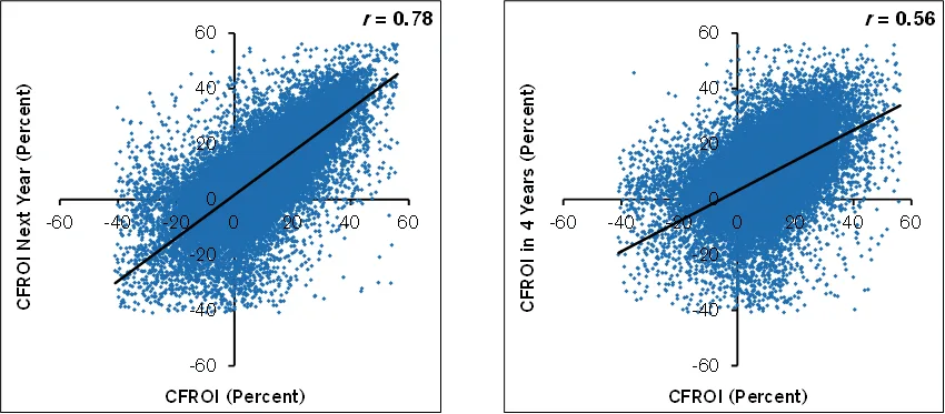
- CFROI shows substantial persistence: global company data from 1983–2015, including failed companies, show correlations of 0.78 over one year and 0.56 over four years.
- Returns regress toward the mean only modestly: over ten years, the CFROI spread between the highest and lowest starting quintiles narrows from 18 to 9 percentage points.
- Sector-specific base rates trade smaller sample sizes for greater relevance, helping investors choose appropriate benchmarks and estimate rates of mean reversion.
There is modest regression toward the mean. The spread from the highest to the lowest quintile shrinks from 18 to 9 percentage points.
Sector Returns and Persistence
- Cash flow return on investment (CFROI) is more persistent in consumer staples than in energy: one-year correlations are 0.89 versus 0.64, and four-year correlations are 0.78 versus 0.35.
- Stable consumer demand supports longer-lasting returns, while exposure to commodity markets is associated with faster regression toward the mean.
- Compounding one-year correlations can overstate long-term mean reversion. For consumer staples, an initial return spread of 10 percentage points implies a four-year spread of 6.3 points using the one-year correlation, versus 7.8 using the observed four-year correlation.
- Across ten sectors studied from 1983–2015, consumer-oriented sectors generally rank highest in four-year return persistence, while commodity-exposed sectors tend to rank lowest.
- Persistence also varies in stability over time: the four-year correlation has a standard deviation of only 0.04 for consumer staples, compared with 0.12 for energy, making sector-specific assumptions important for forecasting.
So using a one-year correlation coefficient overstates the rate of regression toward the mean.
How Corporate Returns Regress
- Excess cash flow returns on investment (CFROI) regress toward sector averages at different speeds: four-year correlations range from 0.78 for consumer staples, indicating greater persistence, to 0.35 for energy, indicating faster regression.
- Forecasting corporate performance requires estimating not only the speed of regression but also the average toward which returns move, since sector averages can change over time.
- From 1983–2015, consumer staples averaged a 9.3% CFROI with a standard deviation of 0.6 percentage points, while energy averaged 4.9% with a standard deviation of 1.7 percentage points.
- Energy’s lower, more volatile returns help explain its faster regression and lower valuation multiples; consumer staples’ higher, steadier returns are associated with higher multiples.
- Percentile bands reveal the spread of company returns within sectors, while the coefficient of variation measures volatility relative to average returns; this ratio was 0.07 for consumer staples versus 0.34 for energy.
For every 100 basis points of CFROI, there’s much more variance in energy than in consumer staples.
Sector Returns and Mean Reversion
- Forecasting cash flow return on investment (CFROI) requires identifying sector-specific drivers of average returns, such as oil prices for energy companies or regulation for financial firms.
- Historical four-year correlations help estimate the rate of mean reversion: consumer staples show greater persistence in returns, while energy exhibits stronger regression toward the mean. These patterns apply to populations, not necessarily individual companies.
- For sectors with stable average CFROIs, such as consumer staples and consumer discretionary, historical averages offer reasonable targets for mean reversion.
- For volatile sectors, analysts should adjust historical averages to reflect mid-cycle profitability, recognizing that structural changes can alter even that benchmark.
- Whether elevated aggregate U.S. profit margins will decline depends on changes in underlying drivers—including labor costs, depreciation, financing costs, and taxes—not simply on mean reversion among individual companies.
Remember that regression works on a population, not necessarily on every individual company.
CFROI Persistence Across Sectors
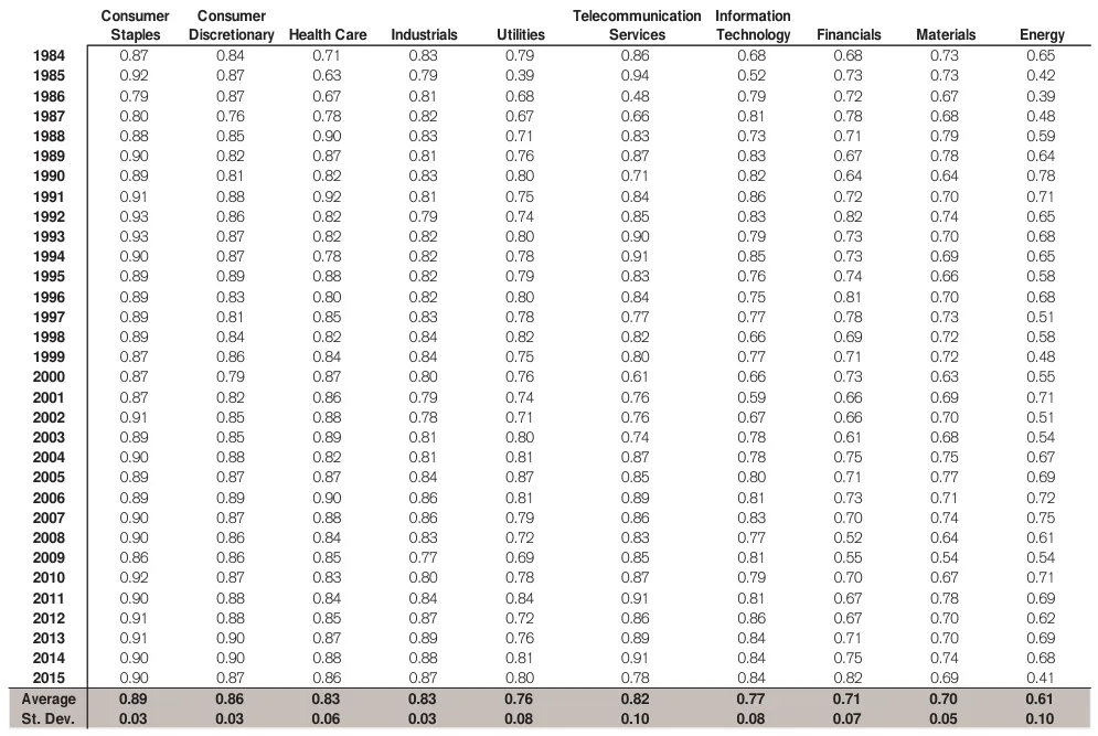
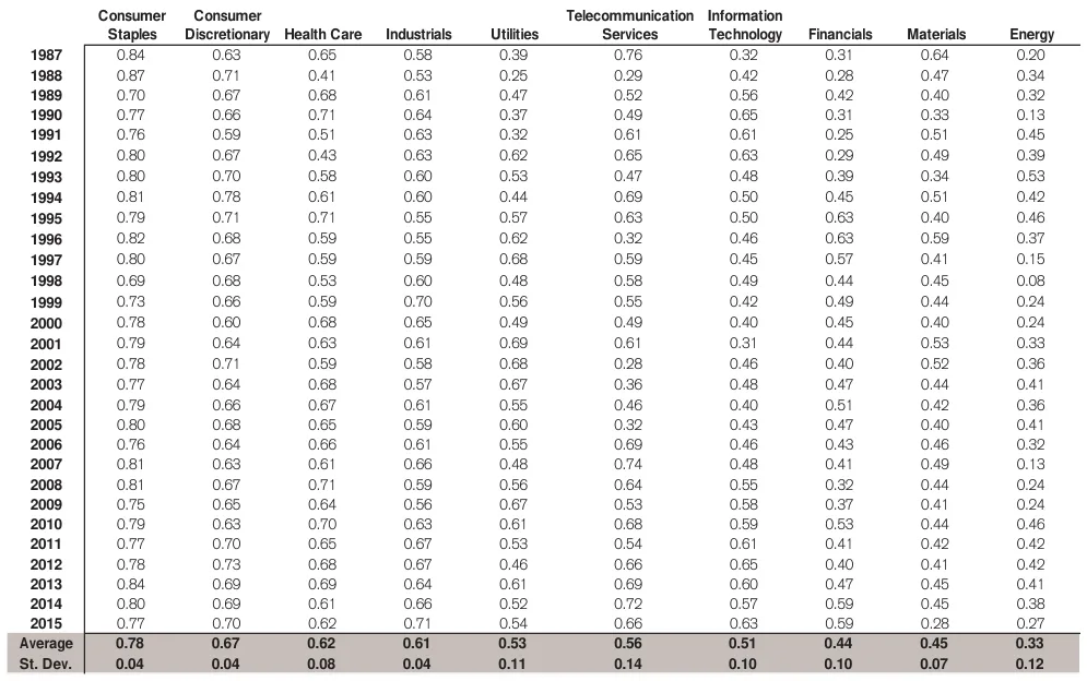
- The exhibits compare CFROI correlation coefficients across ten sectors using global company data from 1983–2015, examining both year-over-year and four-year relationships.
- Consumer staples has the strongest average year-over-year correlation at 0.89, followed by consumer discretionary at 0.86; both have low standard deviations of 0.03.
- Energy has the weakest average annual correlation at 0.61. Energy and telecommunications have the greatest variability in annual correlations, each with a standard deviation of 0.10.
- The four-year observations shown, covering 1987–1994, generally have lower correlations than the annual figures, suggesting that CFROI persistence weakens over longer horizons.
- The sample includes both surviving and defunct companies with scaled market capitalizations of at least $250 million, and observations are Winsorized at the 1st and 99th percentiles to limit extreme values.
Global companies, live and dead, with market capitalizations of $250 million-plus scaled; Winsorized at 1st and 99th percentiles.
Historical Sector CFROI
- Appendix B presents historical sector CFROI data for 1983–2015, providing a basis for comparing returns across industries and over time.
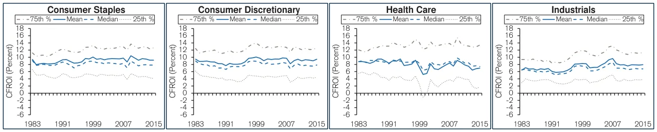
- Exhibit 10 charts mean CFROI for ten sectors, including consumer staples, health care, information technology, financials, and energy.
- Exhibit 11 adds median CFROI and the 25th and 75th percentiles, showing the spread of company returns within each sector rather than averages alone.
- The charts use Credit Suisse HOLT data covering both surviving and defunct global companies, with a stated market-capitalization threshold of $250 million-plus scaled; values are winsorized at the 1st and 99th percentiles.
- The opening table fragment reports annual values, averages, and standard deviations for ten unlabeled series; without column headings, those figures cannot reliably be assigned to specific sectors or metrics.
Plotting the percentiles allows you to see the dispersion in CFROI for the sector.
Investing Under Pressure
- A sharp drop in a portfolio stock can provoke frustration, anger, worry, and shame—emotions that undermine sound investment decisions.
- These “man overboard” moments demand urgent attention and often interrupt several investment professionals as they work out how to respond.
- Checklists offer a framework for decisions under pressure: DO-CONFIRM checks work performed from memory, while READ-DO directs actions step by step.
- READ-DO checklists are especially useful during stressful events because they reduce emotional interference, analytical demands, and decision paralysis.
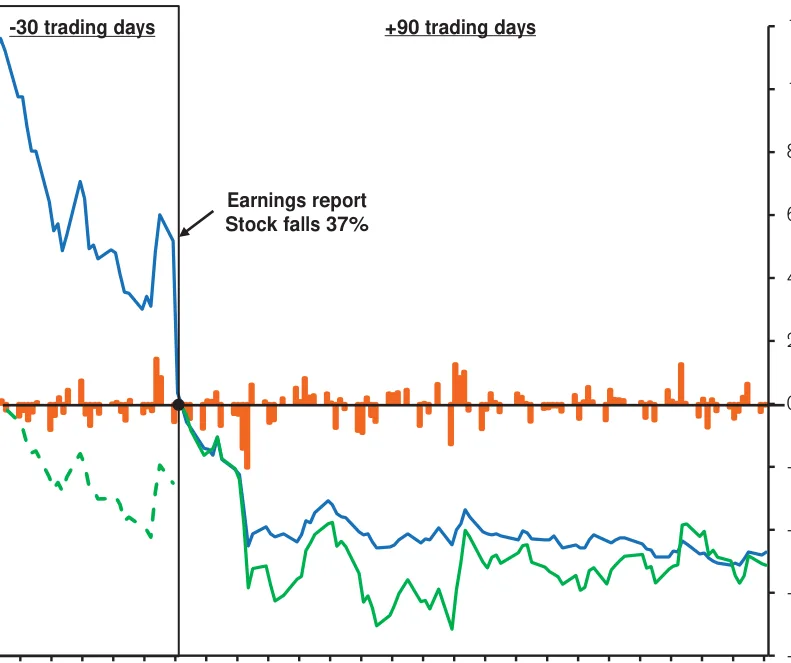
- The report aims to guide buy, hold, or sell decisions after a stock falls at least 10 percent relative to the S&P 500 in a single day.
You can think of your emotional state and the ability to make good decisions as sitting on opposite sides of a seesaw. If your state of emotional arousal is high, your capacity to decide well is low.
After Sharp Stock Declines
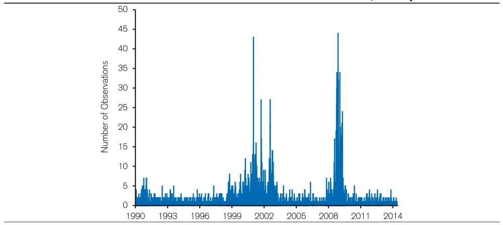
- More than 5,400 relative stock-price declines of at least 10% occurred from January 1990 through June 2014, with roughly 40% clustered in bubble periods; despite their recurrence, few investment firms have a systematic response.
- The study measures subsequent performance over 30, 60, and 90 trading days using cumulative abnormal returns—returns above or below expectations based on the S&P 500 and adjusted for risk.
- Earnings releases account for about one-quarter of the sample, and disappointing earnings announcements generally lead to worse subsequent abnormal returns than other announcements.
- To make base rates more relevant, the analysis groups stocks by sector-relative momentum, valuation, and quality, incorporating cash-flow returns, earnings revisions, price trends, relative cheapness, and value creation.
- Results are broadly consistent with and without bubble periods: corresponding average returns have the same direction more than 80% of the time for earnings announcements and nearly 90% for other events.
These sharp drops happen frequently enough that they deserve a thoughtful process to deal with them but infrequently enough that few investment firms have developed such a process.
Base Rates After Selloffs
- Refining a reference class makes historical base rates more relevant to a particular stock, but reduces sample size, creating a trade-off between fit and statistical support.
- Average stock returns conceal substantial uncertainty: most distributions have medians below their means and standard deviations of 35–45 percent, so averages should not be treated as predictions.
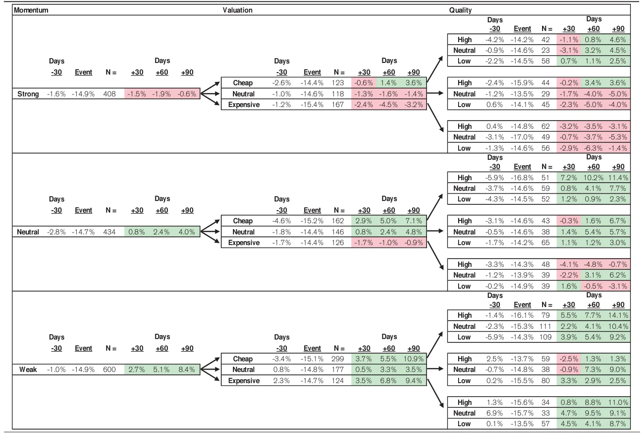
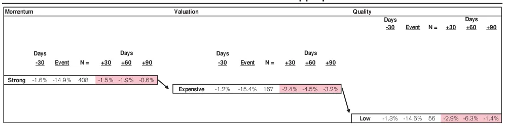
- For a portfolio stock falling at least 10 percent relative to the S&P 500, the checklist first distinguishes earnings from non-earnings announcements, then considers momentum, valuation, and quality.
- In the earnings-event example, 408 strong-momentum stocks fell an average of 14.9 percent on the event day and subsequently underperformed the market by 1.9 percent over 60 trading days.
- Adding expensive valuation narrows the example to 167 stocks with a 60-day abnormal return of -4.5 percent; adding high quality reduces it to 62 stocks with a return of -3.5 percent. The checklist offers immediate guidance while investors reassess the investment.
While our summary figures show a tidy average, recognize that the figure belies a rich distribution.
Rebounds After Sharp Declines
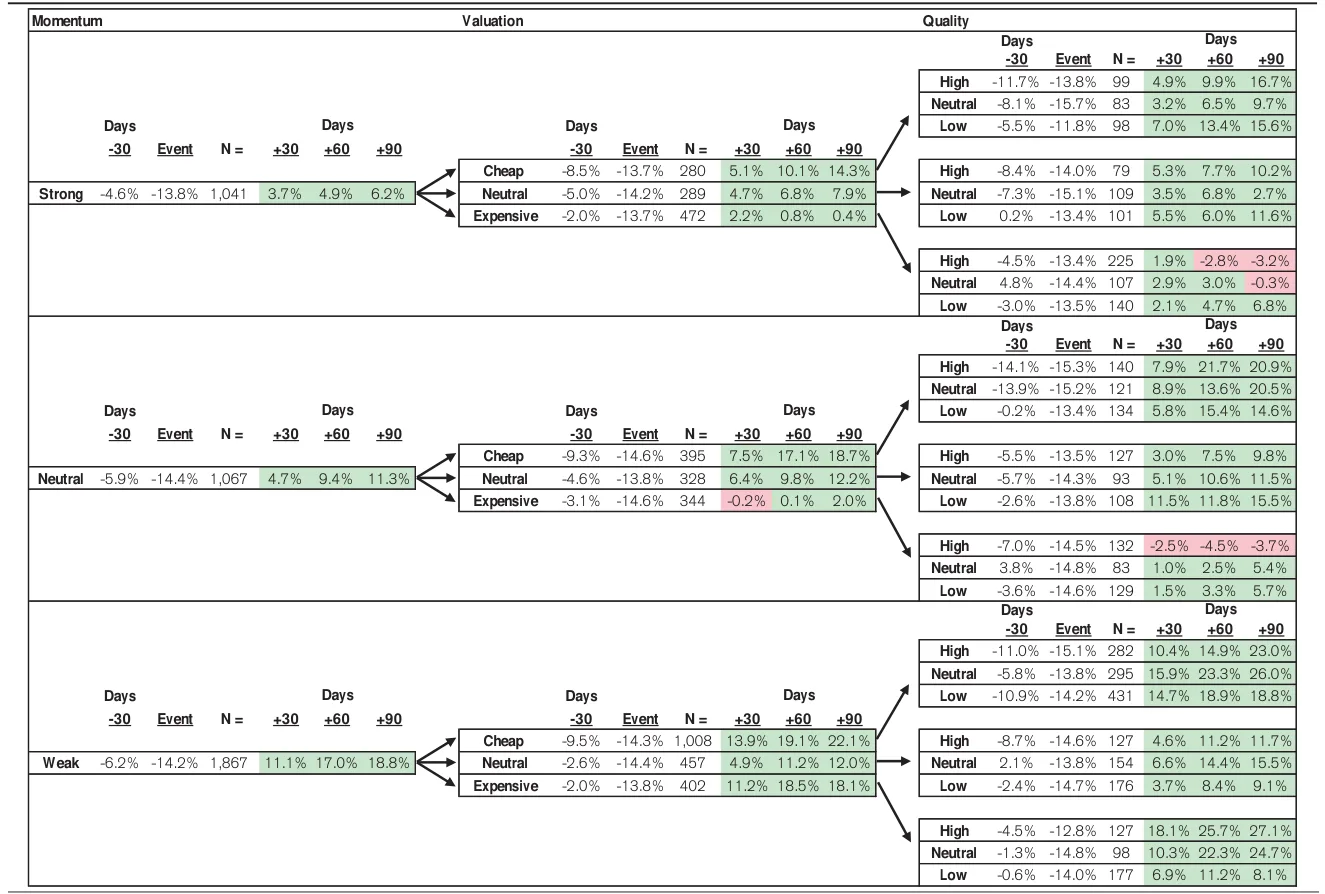
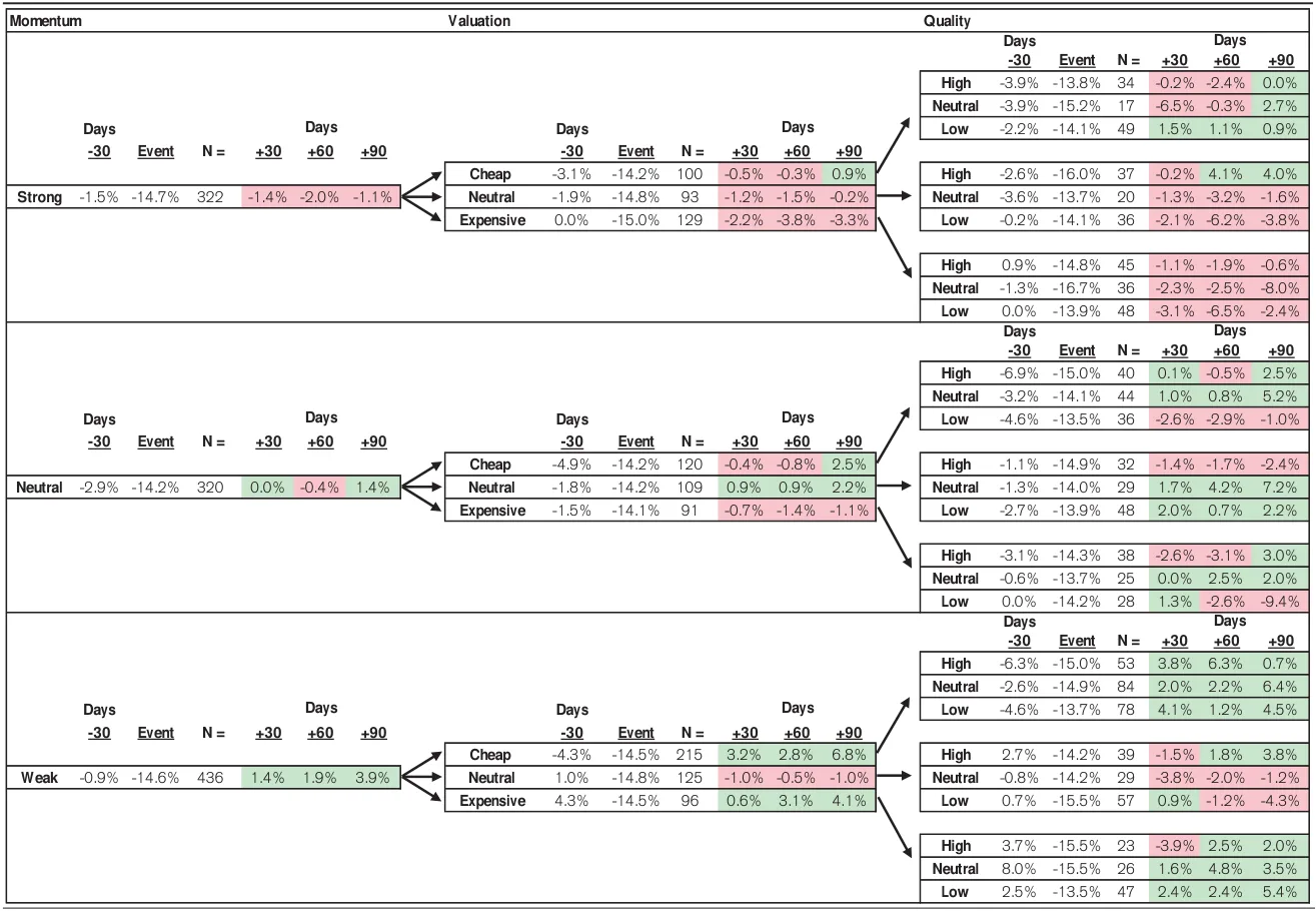
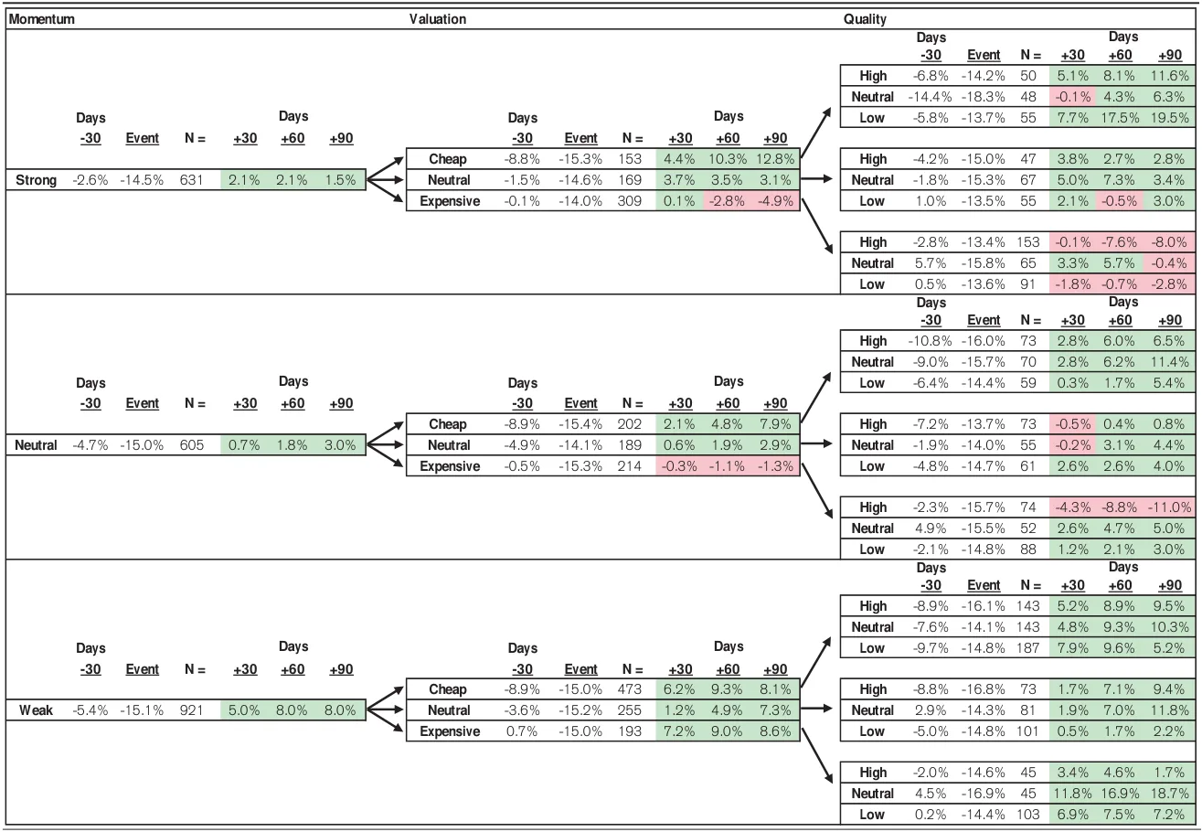
- The exhibits compare abnormal stock returns around earnings and non-earnings events, grouping stocks by prior momentum, valuation, and quality and tracking performance through 90 days afterward.
- Similar event-day losses lead to very different subsequent outcomes. After earnings events, strong-momentum stocks average a −0.6% abnormal return over 90 days, versus +8.4% for weak-momentum stocks.
- Cheap stocks generally recover more strongly than expensive stocks. Following earnings events, cheap stocks with weak momentum gain 10.9% over 90 days, compared with 3.6% for cheap stocks with strong momentum.
- The displayed non-earnings groups show stronger recoveries than their earnings-event counterparts. Cheap stocks with neutral momentum gain 18.7% over 90 days after non-earnings events, versus 7.1% after earnings events.
- Quality does not produce a uniform ranking of recoveries across groups. The tables suggest that the combination of event type, momentum, valuation, and quality is more informative than any single characteristic.
Note: The abnormal return for the event reflects only the day of the event.
Symantec’s Post-Shock Recovery
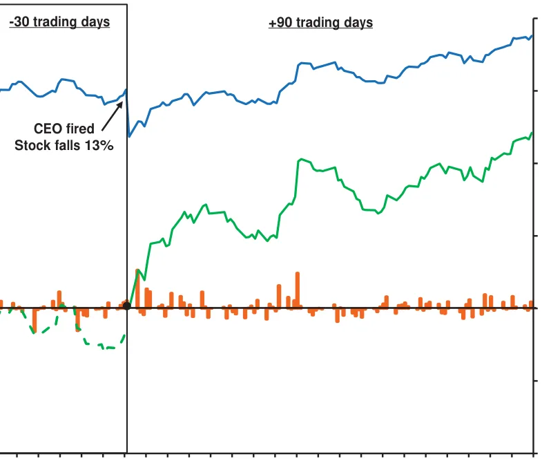
- Symantec shares fell 12.9% on March 21, 2014, after the company announced CEO Steve Bennett’s dismissal; the S&P 500 declined just 0.3%, and the event was unrelated to earnings.
- The analysis measures stock performance using cumulative abnormal return (CAR), subtracting the expected market-related return from the stock’s actual return.
- Expected returns are calculated using the S&P 500’s total return multiplied by the stock’s beta, estimated through a regression of the preceding 60 months of monthly returns.
- Symantec’s beta was approximately 0.8, producing an expected return of about 1.0% over the 30 trading days after the event; its actual return of 10.3% therefore yielded a CAR of 9.3%.
- The subsequent 90-day recovery illustrates how a sharp, company-specific selloff can offer an investment opportunity; the case study proposes examining a checklist to assess whether that opportunity was identifiable in real time.
It’s evident that buying Symantec on the day after this event would have yielded good returns in the subsequent 90 days.
Base Rates After Declines
- For a stock-price event unrelated to a scheduled earnings release, the analysis uses momentum, valuation, and operational quality to identify an appropriate historical reference class.
- HOLT factor scores should be taken on the event date, before overnight price adjustments; scores of 66–100 indicate favorable characteristics, 0–33 unfavorable characteristics, and 34–65 neutral characteristics.
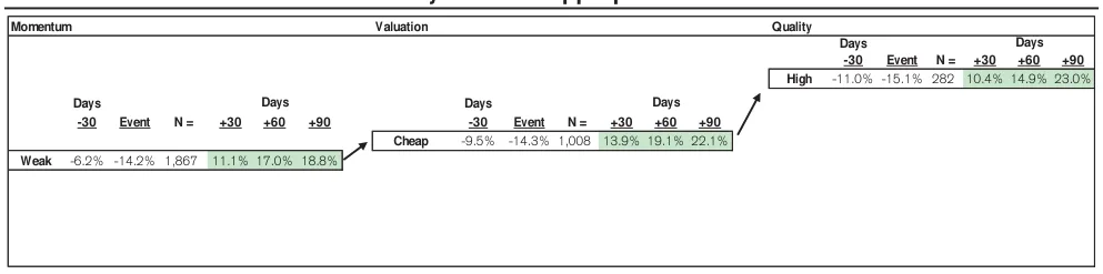
- Symantec’s weak momentum (23), cheap valuation (80), and high quality (71) place it in a reference class containing 282 historical events.
- That reference class produced average cumulative abnormal returns of 10.4%, 14.9%, and 23.0% over the following 30, 60, and 90 trading days, suggesting a purchase the day after the decline.
- Symantec’s subsequent abnormal returns—9.3%, 15.4%, and 24.2%—closely matched those historical averages, but wide return distributions and means above medians underscore the uncertainty hidden by averages.
While the results are consistent with the base rate, we must reiterate that the averages belie a more complex distribution.
Assessing Tenet’s Earnings Collapse
- Charts covering 282 events show an average event-day abnormal return of −15.1%, followed by positive average cumulative abnormal returns of 10.4%, 14.9%, and 23.0% at 30, 60, and 90 days, respectively, with substantial variation.
- On November 4, 2008, Tenet Healthcare reported disappointing scheduled earnings; its stock fell 36.7% even as the S&P 500 rose 4.1%.
- Tenet had already posted a −25.2% cumulative abnormal return before the announcement and continued to decline afterward, illustrating a case in which selling after a sharp loss would have made sense.
- The assessment checklist first identifies the event as a scheduled earnings release, then uses momentum, valuation, and operational quality to select an appropriate reference class.
- Tenet’s factor scores combined barely strong momentum (66) with expensive valuation (9) and low quality (4). Its momentum remained strong because of relative performance over the preceding 52 weeks, despite recent weakness.
This is a case where selling Tenet Healthcare stock, notwithstanding the weak results, would have made sense.
Trading After Sharp Drops
- Historical base rates offer a systematic guide to buying, selling, or holding after a sharp stock-price decline, complementing fundamental analysis and helping counter emotional reactions.
- Weak momentum before a decline signals a buying opportunity following either earnings or non-earnings events; cheap valuation and strong company quality generally strengthen the signal.
- Following earnings releases, the combination of strong prior momentum and expensive valuation indicates selling, regardless of company quality.
- Following non-earnings events, abnormal returns are generally positive, but strong or neutral momentum combined with expensive valuation and high quality produces the strongest sell signal.
- Tenet Healthcare illustrates both the usefulness and limits of base rates: its characteristics suggested selling, but its subsequent abnormal losses far exceeded the reference-class averages, underscoring that forecasts remain probabilistic.
Further, large price drops almost always evoke a strong emotional reaction, which complicates the process of decision making even more.
Base Rates After Selloffs
- Sharp stock declines heighten emotions and complicate investment decisions; historical base rates provide a more grounded way to assess what may happen next.
- The exhibits compare cumulative abnormal returns around earnings and non-earnings selloffs outside the bubble period, grouping stocks by momentum, valuation, and quality.
- After earnings-related declines, weak-momentum stocks gained 3.9% in abnormal returns over 90 days, while strong-momentum stocks lost another 1.1%, showing that prior strength did not guarantee recovery.
- Valuation meaningfully differentiated outcomes: among strong-momentum stocks experiencing non-earnings declines, cheap stocks gained 12.8% over 90 days, whereas expensive stocks lost 4.9%.
- Quality also varied within these categories: cheap, strong-momentum stocks with low quality gained 19.5% after non-earnings declines, illustrating why recovery expectations should consider combinations of characteristics rather than one attribute alone.
Deciding what to do with a stock following a sharp decline is particularly difficult because emotions tend to run high after those events.
Defining Stock Selection Factors
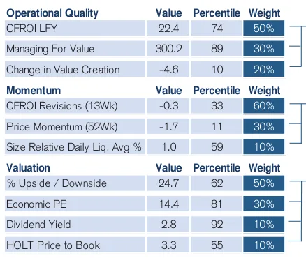
- Momentum gauges market sentiment through changes in expected cash flow return on investment (CFROI), stock-price performance, and trading liquidity.
- The momentum score weights 13-week CFROI revisions at 60%, 52-week price momentum at 30%, and daily liquidity at 10%, emphasizing improving earnings expectations.
- Valuation compares a stock’s current market price with its warranted value under the HOLT framework, classifying greater potential upside as cheaper valuation.
- The valuation score combines warranted-price upside (50%), Economic P/E (30%), value-to-cost ratio (10%), and dividend yield (10%).
- HOLT standardizes financial figures and adjusts for factors such as inflation, capitalized R&D, leases, and pension obligations to make valuations more comparable across companies, industries, and accounting systems.
Stocks with the most upside are cheap, and those with the least upside, or downside, are expensive.
Quality Scores and Returns
- HOLT’s operational-quality score weights the latest fiscal year’s cash flow return on investment (CFROI) at 50%, managing for value at 30%, and change in value creation at 20%.
- Growth creates value when CFROI exceeds the cost of capital and destroys value when it falls below that threshold; quality therefore depends on profitable expansion or a willingness to shrink unprofitable businesses.
- The Symantec scorecard illustrates how operational quality, momentum, and valuation combine into an overall assessment, with detailed factor scores available through HOLT Lens.
- The appendix examines distributions of cumulative abnormal stock returns around non-earnings-announcement events, including bubble periods, reporting sample sizes and descriptive statistics.
- Successively filtering cases for weak momentum, cheap valuation, and high quality narrows the comparison group sharply: valuation nearly halves the initial sample, and adding quality leaves just over one-quarter of the preceding group. Returns are examined before, during, and up to 90 trading days after each event.
Growth in businesses that earn a CFROI in excess of the cost of capital is value creating, while growth in businesses with a negative spread destroys value.
Post-Event Return Distributions
- The Symantec case-study charts show negative abnormal returns before and during an event, followed by positive average cumulative abnormal returns over the next 30, 60, and 90 days.
- In the initial sample of 1,867 observations, the average event-day abnormal return is −14.2%; average cumulative abnormal returns afterward reach 11.1% at 30 days and 18.8% at 90 days.
- Filtering for weak momentum and cheap valuation reduces the sample to 1,008 observations and produces higher average subsequent returns: 13.9% at 30 days, 19.1% at 60 days, and 22.1% at 90 days.
- Adding high quality narrows the sample to 282 observations. Average returns are lower at 30 and 60 days than for the cheap-valuation group, but rise to 23.0% at 90 days, with a median of 18.2%.
- Post-event outcomes vary widely: 90-day standard deviations range from 46.0% to 50.4%, and means exceed medians in every post-event distribution. Positive averages therefore mask substantial uncertainty and asymmetric outcomes.
Weak Momentum, Cheap Valuation, High Quality
Managing Investment Euphoria
- A sharp stock-price gain can trigger pride and excitement that impair judgment, making emotional discipline essential even when investments succeed.
- The authors call this a “celebrating the summit” moment: just as climbers can let their guard down before a dangerous descent, investors can underestimate the difficulty of deciding when to sell.
- Checklists help counter emotional decision-making and paralysis. READ-DO checklists, which prescribe actions step by step, are especially useful during heightened emotional arousal.
- The report examines whether to buy, hold, or sell after a stock outperforms the S&P 500 by at least 10 percentage points in one day, excluding gains tied to announced mergers and acquisitions.
- Roughly 6,800 such events occurred from January 1990 through mid-2015, with 36 percent clustered in bubble periods. A typical fund manager might face 5–15 annually in calm years and more than 100 in volatile years, yet few firms have a formal process for handling them.
He points out that mountain climbers commonly celebrate too much at the peak. This causes them to let their guard down just as they are approaching the part of the expedition that may be the most challenging.
After Sharp Stock Gains
- The study measures stock performance after large price jumps using cumulative abnormal returns: returns above those expected from risk-adjusted S&P 500 performance over 30, 60, and 90 trading days.
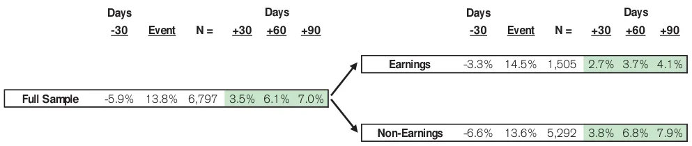
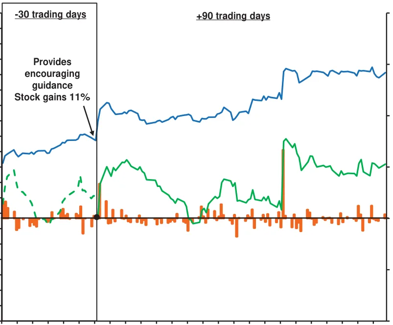
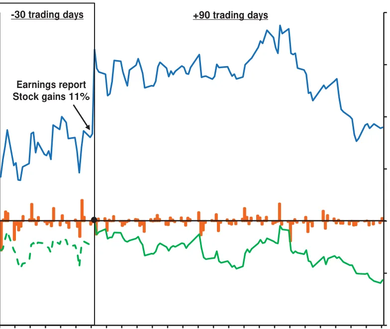
- Across 6,797 events, stocks underperformed the market by 5.9 percentage points in the preceding 30 days, jumped 13.8 percentage points on the event date, and subsequently earned average abnormal returns of 7.0% over 90 trading days.
- Non-earnings events produced stronger subsequent gains than earnings announcements: average 90-day abnormal returns were 7.9% versus 4.1%, respectively.
- Positive earnings surprises tend to be followed by further stock price gains, consistent with the established phenomenon of post-earnings-announcement drift.
- To make these base rates more useful, the analysis also classifies companies by sector-relative momentum, valuation, and quality, incorporating cash-flow return forecasts, stock price trends, relative cheapness, and consistent value creation.
The first thing to note is that weak relative stock price results generally precede the large positive moves.
Interpreting Stock Surge Base Rates
- Refining a reference class makes historical base rates more relevant to a particular stock, but reduces the sample size and requires balancing specificity against available evidence.
- Average abnormal returns conceal substantial uncertainty: most distributions are right-skewed, with medians below means and standard deviations typically between 30 and 45 percent.
- For a portfolio stock that rises at least 10 percent relative to the S&P 500 for reasons unrelated to announced M&A, the checklist examines announcement type, prior momentum, valuation, and quality.
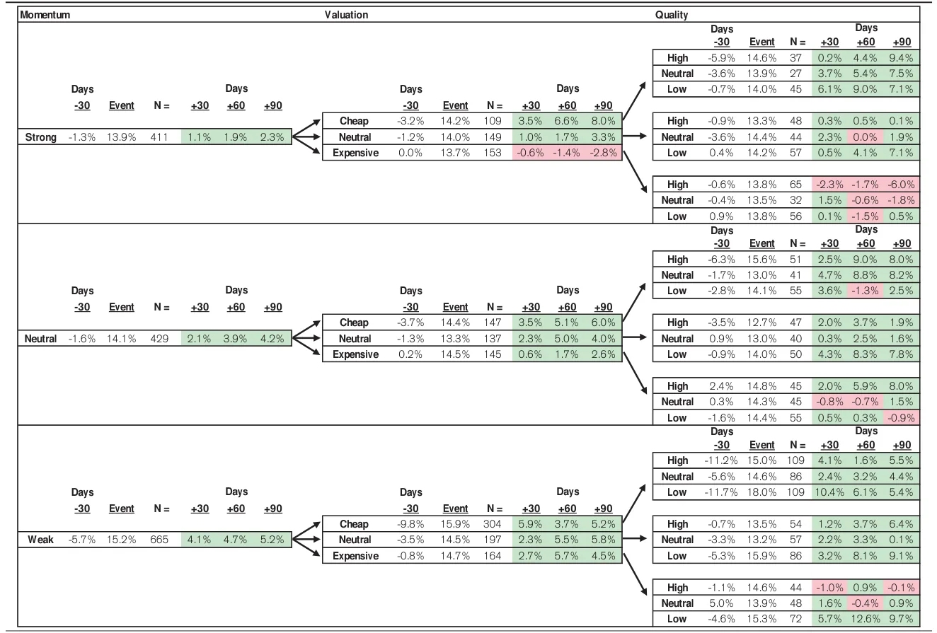
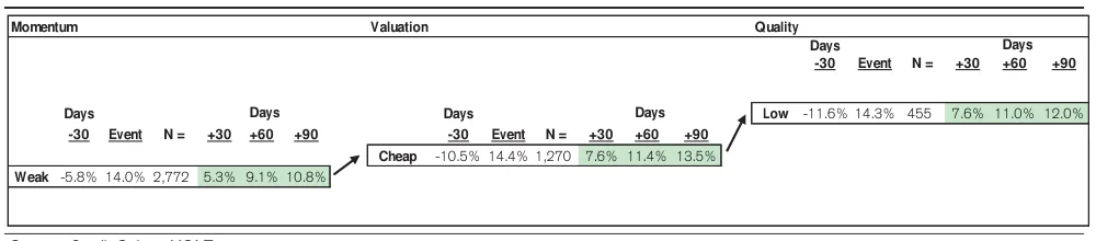
- In the example, 665 stocks with weak momentum that jumped on earnings news subsequently earned average cumulative abnormal returns of 4.1 percent over 30 trading days, 4.7 percent over 60, and 5.2 percent over 90.
- Adding expensive valuation narrows the example to 164 cases with a 5.7 percent average 60-day abnormal return; adding low quality reduces it to 72 cases with a 12.6 percent return, illustrating how refinement changes both expectations and sample size.
- The checklist provides immediate, probabilistic guidance while giving investment teams up to 90 trading days to reassess a stock’s merits, rather than treating historical averages as guaranteed outcomes.
While our summary figures show a tidy average, recognize that the figure belies a rich distribution.
Returns After Price Jumps
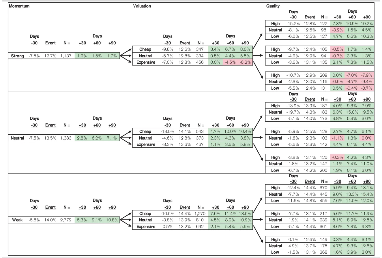
- The exhibits compare cumulative abnormal stock returns around earnings and non-earnings events, separating stocks by momentum, valuation, and quality and tracking performance through 90 days afterward.
- Cheap stocks outperform expensive stocks at the 90-day horizon in every fully displayed momentum group across both exhibits, suggesting valuation helps distinguish lasting gains from temporary jumps.
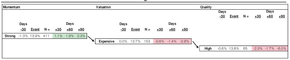
- Among strong-momentum stocks, cheap shares gain another 8.0% after earnings events and 8.6% after non-earnings events by day 90; expensive shares lose 2.8% and 6.2%, respectively.
- Strong prior momentum does not guarantee stronger follow-through: after earnings events, the weak-momentum group gains 5.2% by day 90, compared with 2.3% for the strong-momentum group.
- Event-day abnormal returns are reported separately from subsequent cumulative returns. Large initial jumps can therefore coexist with weak or negative later performance.
Note: The abnormal return for the event reflects only the day of the event.
Harman’s Post-Event Returns
- At its August 8, 2013 investor day, Harman issued financial guidance for fiscal 2014 and 2016. Its stock jumped 10.7% while the S&P 500 fell 0.4%, making this a notable non-earnings event.
- The analysis measures performance using cumulative abnormal return (CAR), separating a stock’s actual return from the return expected given its market exposure.
- Expected returns equal the S&P 500’s total return multiplied by the stock’s beta. Beta is estimated from the preceding 60 months of monthly returns and updated monthly.
- Over the 90 trading days following the event, Harman returned 25.3%. Subtracting its beta-adjusted expected return of 13.5% produced a CAR of 11.8%.
- Harman’s continued gains illustrate that a large initial price jump need not exhaust an investment opportunity; the authors use the case to introduce a checklist for assessing such situations in real time.
It’s evident that buying Harman on the day after this event would have yielded good returns in the subsequent 90 days.
Applying Stock Return Base Rates
- The Harman case illustrates how to select a historical reference class after a stock-price jump unrelated to a scheduled earnings release.
- Factor scores should be taken on the event date, before overnight updates incorporate the price gain. Harman scored weak on momentum, cheap on valuation, and low on operational quality.
- The resulting reference class of 455 events had average cumulative abnormal returns of 7.6% after 30 trading days, 11.0% after 60 days, and 12.0% after 90 days, suggesting a purchase the day after the jump.
- Harman’s actual cumulative abnormal returns were −1.0%, 15.5%, and 10.5% over those periods, broadly consistent with the historical pattern despite short-term underperformance.
- Positive averages conceal substantial uncertainty: mean returns exceeded medians, and standard deviations rose from about 30% at 30 days to 45% at 90 days, underscoring the wide range of possible outcomes.
While the results are consistent with the base rate, we must reiterate that the averages belie a more complex distribution.
Grainger’s Post-Earnings Reversal
- W.W. Grainger’s shares jumped 11.4% after strong scheduled earnings on July 18, 2012, compared with a 0.7% rise in the S&P 500.
- The analysis classifies the event using a checklist and factor scores: strong momentum (80), expensive valuation (19), and high operational quality (68).
- Grainger’s closest reference class, comprising 65 historical events, had negative cumulative abnormal returns of −2.3%, −1.7%, and −6.0% over 30, 60, and 90 trading days, supporting a decision to sell.
- Grainger subsequently underperformed, with cumulative abnormal returns of −5.2%, −0.9%, and −11.3% over those same horizons, broadly consistent with the historical warning.
- Base rates offer a probabilistic guide rather than a certain forecast: individual outcomes vary within each reference class.
Once again, note that there is a distribution of returns for this reference class, and the best we can do is make a probabilistic assessment.
After a Stock Surge
- Sharp stock-price gains can trigger emotions that undermine judgment; historical base rates provide a systematic complement to fundamental analysis when deciding whether to buy, sell, or hold.
- Following earnings announcements, stocks with weak or neutral prior momentum show a clear buy signal, strengthened by cheap or neutral valuations.
- For non-earnings events, weak prior momentum produces an even stronger buy signal, especially when combined with cheap valuations and high or neutral company quality.
- Strong prior momentum combined with expensive valuation is the clearest sell signal across both earnings and non-earnings events, particularly for high- or neutral-quality companies.
- Although post-event abnormal returns are largely positive for non-earnings events, these stocks had previously underperformed the market by nearly seven percentage points, highlighting the importance of context.
Mountain climbers run a risk of “celebrating the summit,” enjoying the pleasure without considering the rest of the journey.
Harman Return Distributions
- The Harman case study progressively narrows its comparison group using weak momentum, cheap valuation, and low quality, illustrating the trade-off between specificity and sample size.
- The weak-momentum group contains 2,772 cases: mean abnormal returns were −5.8% over the preceding 30 trading days and 14.0% on the event day.
- Adding cheap valuation reduces the sample to 1,270 cases. These stocks had a larger average pre-event decline of −10.5%, but a similar event-day gain of 14.4%.
- The cheap, weak-momentum group shows higher average subsequent cumulative abnormal returns: 7.6%, 11.4%, and 13.5% at 30, 60, and 90 trading days, versus 5.3%, 9.1%, and 10.8% for weak momentum alone.
- Both groups show considerable uncertainty: 90-day standard deviations exceed 40%, and means exceed medians. Adding low quality leaves just over one-third of the second group's sample, but its return statistics are not shown in this excerpt.
The sample size is just over one-third of the prior branch.
Event Returns and Sources
- Charts covering 455 observations show a mean cumulative abnormal return of −11.6% in the 30 days before an unspecified event, followed by a mean abnormal return of 14.3% at the event.
- Mean cumulative abnormal returns remain positive at 30, 60, and 90 days after the event, reaching 7.6%, 11.0%, and 12.0%, respectively.
- Post-event outcomes become more dispersed over time: standard deviation rises from 32.0% at 30 days to 46.1% at 90 days, indicating substantial variation behind the positive averages.
- The introduction’s endnotes cite research on base-rate neglect, executive optimism, statistical prediction, and the outside view, documenting the book’s foundations in decision science.
- A technical note explains that a shrinkage factor can range from −1 to 1; a value of −1 implies that a good result is followed by an equally large poor result.
A shrinkage factor of -1.0 would suggest that a good result of a certain magnitude is followed by a poor result of similar magnitude.
Forecasting and Corporate Growth
- This section consists primarily of references supporting discussions of investing, optimism, forecasting biases, and corporate growth, rather than presenting a new argument.
- Cited research examines persistent optimism, entrepreneurs’ expectations of success, analyst forecast biases, and managerial miscalibration, highlighting the relevance of judgment errors to business decisions.
- References on corporate mortality and longevity accompany the explicit observation that most public companies “die” through mergers and acquisitions.
- Other sources address company growth patterns, capital investment and stock returns, and the persistence of growth rates—topics relevant to evaluating corporate performance.
- A methodological note states that the top and bottom two percent of growth rates are winsorized; exceptionally high growth rates generally involve very small companies or substantial merger-and-acquisition activity.
Most public companies “die” as the result of mergers and acquisitions.
Debating the Profitability Premium
- This reference section points to research on value investing, profitability, and market efficiency, including reflections on Benjamin Graham’s legacy.
- Cited work examines the gross profitability premium and the role of company quality in investment returns.
- Some researchers dispute whether gross profit measures earnings better than net income or operating income, arguing that gross profitability and net income have similar predictive power when scaled consistently.
- Another cited study proposes operating leverage as an explanation for the excess returns associated with gross profitability.
- Additional references cover the five-factor asset pricing model and international evidence on the gross profitability effect, situating the debate within broader research on stock returns.
They argue that gross profitability and net income have similar predictive power when they are deflated the same way.
Investment Analysis References
- This section is a bibliography from The Base Rate Book, listing sources rather than presenting a sustained argument or new findings.
- Several references examine analysts’ earnings forecasts, including forecast errors, declining sales, and differences between buy-side and sell-side analysts.
- A recurring research theme is the relationship between operating leverage, cost behavior, earnings, and investment risk.
- Other sources address business strategy and growth, including competitive advantages, total addressable markets, innovation, and industry concentration.
- References on valuation, capital allocation, and market-share objectives broaden the reading list to questions of corporate performance and investment assessment.
“Competitor-oriented Objectives: The Myth of Market Share,”
Financial Performance Research Sources
- This section consists of bibliographic references rather than substantive argument, documenting research used in The Base Rate Book.
- The opening references cover pricing elasticity, forecasting accuracy, operating leverage, capital structure, and corporate cash holdings.
- The operating-profit-margin references highlight debates about rising corporate margins and a “winner take all” economy.
- The earnings-growth references address financial reporting decisions, investor disclosure preferences, earnings guidance, and valuation methods.
- Further citations trace research on the relationship between earnings and stock prices, including the information conveyed by earnings announcements and the effects of mandatory IFRS adoption.
“Profit Margins in a ‘Winner Take All’ Economy,”
Earnings Research and Methodology
- This section consists mainly of references supporting research on earnings, accounting quality, growth rates, and investment analysis, rather than presenting new findings.
- The report’s sample covers the top 1,000 global companies by market capitalization across all sectors since 1950; the early sample is smaller, reaching 1,000 companies by the late 1960s.
- Growth-rate calculations exclude companies with negative net income, a methodological choice that matters when interpreting the report’s results.
- Net income is defined as income before extraordinary items, using Compustat annual data item 18; it includes special items but excludes discontinued operations and extraordinary items presented after taxes.
- The cited literature addresses analyst forecast errors, investor sentiment, earnings persistence, adjusted versus GAAP earnings, and company-growth volatility, establishing the research context for the report.
“Financial Analysts Were Only Wrong by 25%,”
Valuation and Decision Resources
- This section consists mainly of endnotes and a resource list supporting discussions of valuation, emergency decision-making, and managing success.
- HOLT models cash flow return on investment (CFROI) in three stages: a five-year fade based on corporate life cycle, an annual reduction of 10 percent of the remaining economic spread, and a terminal return equal to the cost of capital.
- A methodological caveat notes that a previously presented equation is chiefly appropriate for one-time adjustments, citing research on regression toward the mean.
- References on investment checklists, aviation emergencies, survival, and the outside view connect financial decision-making with methods for handling high-pressure situations.
- The resource list broadens the background reading to strategy, financial statement analysis, industry studies, checklists, and the psychology of happiness.
Managing the Man Overboard Moment
Investment Research Bibliography
- This section of The Base Rate Book is a bibliography, listing books and academic papers rather than presenting arguments or findings.
- The books cover company valuation, shareholder value, competitive strategy, and growth, reflecting the report’s broad grounding in business and investment analysis.
- Works on cognitive biases, counterintuition, and the distinction between skill and luck connect financial judgment with psychology and decision-making.
- References on statistical prediction and research methods highlight the methodological foundations relevant to evaluating investment evidence.
- The articles address operating leverage, cost stickiness, stock-price reversals, market efficiency, and earnings information, alongside questions about optimism and market-share objectives.
“Prescribed Optimism: Is It Right to Be Wrong About the Future?”
Financial Research Bibliography
- This bibliography from The Base Rate Book lists research on investing, accounting, corporate finance, and decision-making rather than presenting arguments or findings directly.
- Several entries examine earnings announcements, alternative earnings measures, and analyst forecasting errors, highlighting the importance of interpreting financial information.
- Studies of post-earnings-announcement drift and stock-price reversals address how quickly and fully markets incorporate information.
- Research on base-rate neglect, managerial miscalibration, and entrepreneurs’ expectations connects financial decisions with potential errors in judgment.
- Other references cover profitability, growth persistence, cash holdings, leverage, and valuation, providing sources for assessing corporate performance and investment prospects.
“Evidence that Stock Prices Do Not Fully Reflect the Implications of Current Earnings for Future Earnings,”
Forecasting and Finance References
- This section is a bibliography from The Base Rate Book, listing research sources rather than presenting arguments or findings.
- Many references examine earnings forecasts, including analyst biases, investor sentiment, and the relative accuracy of management and analyst predictions.
- Other cited works address stock-market overreaction, momentum, profitability, and asset-pricing models, outlining a research foundation for assessing investment returns.
- Research on the psychology of prediction and large-project forecasting connects financial analysis with broader questions about cognitive bias and risk assessment.
- Studies of company mortality, operating leverage, capital structure, and financial reporting broaden the bibliography’s coverage of corporate performance and financial decisions.
“Timid Choices and Bold Forecasts: A Cognitive Perspective on Risk Taking,”
Investment Research Bibliography
- This bibliography section of The Base Rate Book lists research on investing, corporate performance, and decision-making rather than presenting arguments or findings.
- References on market efficiency, stock-price shocks, earnings guidance, and accrual reliability address how financial information relates to stock prices.
- Studies of operating and financial leverage, profitability, and firm growth provide sources for examining corporate risk and performance.
- Behavioral research covers executive optimism, the persistence of hope despite experience, and the use of analogies and an outside view in decision-making.
- Other references address practical investment analysis, including capital allocation, corporate longevity, market-size estimation, useful statistics, and investment checklists.
“Hope Over Experience: Desirability and the Persistence of Optimism,”
Corporate Finance Research Sources
- This closing bibliography section lists research sources for The Base Rate Book, dated September 26, 2016.
- Referenced studies address merger-and-acquisition decisions and patterns in company growth, providing context for evaluating corporate outcomes.
- Other citations examine financial analysts’ forecast errors and explanations for the gross profitability effect in international equity markets.
- The remaining sources cover demand’s sensitivity to price, the relationship between capital investment and stock returns, and stock-picking research.
- The excerpt supplies references rather than findings, so the cited works’ conclusions cannot be established from this section alone.
“Financial Analysts Were Only Wrong by 25%,”
Base Rates Improve Forecasts
- Fundamental investing seeks gaps between the performance implied by an asset’s price and its eventual results; success depends on identifying mispriced expectations, not simply strong performers.
- The most accurate forecasts thoughtfully blend both views, giving more weight to case-specific analysis when skill dominates and to base rates when luck plays a larger role.
The goal is not to pick the winner of the race but rather the horse that has odds that are mispriced relative to its likelihood of winning.
Forecast Biases and Base Rates
- Optimism can encourage perseverance but inflates expectations: although only about half of new businesses survive five years, over 80% of surveyed entrepreneurs put their success odds at 70% or higher.
- Overconfidence makes people more certain than their accuracy justifies and produces forecast ranges that are too narrow; CFOs’ purported 80%-confidence stock-market ranges captured actual outcomes only one-third of the time.
Forecasts are commonly too optimistic and too narrow.
Growth Forecasts Meet Reality
- For companies starting with $4.5–7 billion in sales, none in the historical sample sustained annual sales growth of 45 percent or more for ten years; only 0.2 percent achieved 30–35 percent growth.
- Exceptional short-term growth rarely persists over a decade. Among companies with sales below $325 million, 15.1 percent grew more than 45 percent over one year, versus 2.1 percent on a ten-year annualized basis.
Indeed, you have to go down to 30-35 percent growth to see any companies, and even there it is only one-fifth of 1 percent of the sample.
Gross Profitability Persists
- Gross profitability is highly persistent: correlations with future profitability are 0.95 after one year, 0.89 after three years, and 0.82 after five years.
- Profitability quintiles show little regression toward the mean, with the highest-to-lowest spread narrowing only from 0.54 to 0.49; last year’s profitability is therefore a sensible starting point for forecasts.
Given this stability, a sensible forecast is to start with last year’s profitability and seek reasons to move away from it.
Operating Margins and Value
- ROIC combines profitability with capital velocity. Cost leaders such as Wal-Mart typically pair low margins with high sales relative to invested capital, while differentiated businesses such as Tiffany tend toward high margins and lower capital velocity.
- Operating margins are highly persistent: correlations between current margins and margins one, three, and five years later are 0.91, 0.79, and 0.72, respectively, making current profitability informative about future performance.
FCF is the cash that is distributable to a company’s debtors and equity holders, and hence is the lifeblood of corporate value.
The Perils of Growth Promises
- A test of the 200 highest-earning companies in 1990 supports Buffett’s warning: only 14 of the 162 surviving companies achieved at least 15% annual net income growth during 1990–1999, and none of those 14 exceeded 15% in the following decade.
- Lofty earnings promises can distort executive behavior, encouraging economically unsound decisions and accounting manipulation that may escalate from fudging into fraud.
These can turn fudging into fraud. (More money, it has been noted, has been stolen with the point of a pen than at the point of a gun.)
Trading After Sharp Drops
- Weak momentum before a decline signals a buying opportunity following either earnings or non-earnings events; cheap valuation and strong company quality generally strengthen the signal.
- Tenet Healthcare illustrates both the usefulness and limits of base rates: its characteristics suggested selling, but its subsequent abnormal losses far exceeded the reference-class averages, underscoring that forecasts remain probabilistic.
Further, large price drops almost always evoke a strong emotional reaction, which complicates the process of decision making even more.
Returns After Price Jumps
- Cheap stocks outperform expensive stocks at the 90-day horizon in every fully displayed momentum group across both exhibits, suggesting valuation helps distinguish lasting gains from temporary jumps.
- Strong prior momentum does not guarantee stronger follow-through: after earnings events, the weak-momentum group gains 5.2% by day 90, compared with 2.3% for the strong-momentum group.
Note: The abnormal return for the event reflects only the day of the event.