Generative illustration for Principles of Economics





























































































































Principles of Economics
Overview unavailable.
LibreTexts Economics Overview
- Introduces Principles of Economics as a freely available LibreTexts Open Educational Resource, with licensing guidance for use, printing, adaptation, and remixing.
- Describes LibreTexts’ mission to provide customizable, low-cost open-access educational materials through a collaborative online platform.
- Acknowledges institutional and grant support, including the Department of Education, UC Davis, CSU Affordable Learning Solutions, Merlot, and the National Science Foundation.
- Provides contact and social media information for questions about adoption or adaptation, and notes the text compilation date of 04/16/2025.
- Lists the full table of contents, covering microeconomics, macroeconomics, international economics, public policy, development, appendices, glossary, index, and detailed licensing.
Economics: The Study of Choice
- Economics is defined as a social science that investigates how individuals and societies make decisions among available alternatives.
- The discipline is categorized as a science because it employs a systematic, scientific approach to study human behavior and decision-making.
- The core of economic theory rests on the relationship between scarcity, choice, and the resulting opportunity costs.
- Every economic system must address three fundamental questions: what to produce, how to produce it, and for whom it is produced.
- Scarcity necessitates choice, meaning that selecting one option inherently requires the sacrifice of another alternative.
Economics is a social science that examines how people choose among the alternatives available to them.
The Reality of Scarcity
- Human wants are unlimited while the resources available to satisfy them are finite.
- Economics is defined by the necessity of making choices between competing alternatives.
- A good is considered scarce if choosing one use for it requires giving up another use.
- Even seemingly infinite resources like air are scarce because they have alternative uses, such as breathing versus pollution.
- Free goods, like gravity, are rare because one person's use does not diminish the availability for others.
- The increasing utilization of outer space demonstrates how free goods can become scarce as human activity expands.
The fact that gravity is holding you to the earth does not mean that your neighbor is forced to drift up into space!
Scarcity and Opportunity Cost
- Every society must address three fundamental questions: what to produce, how to produce it, and for whom it should be produced.
- Scarcity necessitates trade-offs, such as choosing between better education and healthcare or preserving wilderness versus industrial land use.
- The concept of opportunity cost is defined as the value of the best alternative forgone when making a specific choice.
- Opportunity cost differs from purchase price because it includes the value of time and other non-monetary resources sacrificed.
- The most significant cost of a college education is often the value of the time spent studying rather than the direct cost of tuition.
- A good is considered scarce if choosing one alternative requires that another must be surrendered.
Opportunity cost is the value of the best alternative forgone in making any choice.
Scarcity and Opportunity Cost
- Opportunity cost is defined as the value of the best alternative forgone when making a specific choice.
- Economic decisions involve trade-offs between competing interests, such as environmental preservation versus urban housing development.
- The consumption of exhaustible resources like oil imposes an opportunity cost on future generations who will no longer have access to those resources.
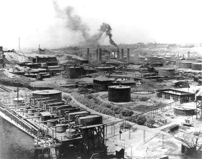
- As easily accessible 'light crude' oil diminishes, the global economy is shifting toward 'heavy crude' found in sandy soils.
- Extracting heavy crude from oil sands is significantly more expensive and causes greater environmental degradation than traditional drilling.
- The transition to heavier oil resources represents a new geological reality where energy production requires more labor, capital, and ecological sacrifice.
The oily sand is then hauled off in two-story dump trucks which, when filled, weigh more than a Boeing 747.
The Cost of Heavy Crude
- Extracting heavy crude oil from Alberta's oil sands costs $25 per barrel, significantly higher than the $6 required for light crude.
- The environmental impact is severe, with heavy crude production generating three times the greenhouse gas emissions of light crude.
- By 2015, the town of Fort McMurray was projected to emit more greenhouse gases than the entire nation of Denmark.
- Economic viability for oil sands shifted in the mid-2000s as global oil prices surged from $12 to over $70 per barrel.
- The development creates a sharp conflict between economic benefits and the permanent destruction of boreal forest ecosystems.
- The situation illustrates the economic concept of opportunity cost, where resource use requires choosing between competing values like industry and preservation.
“You see a lot of the land dug up, a lot of the boreal forest struck down and it’s upsetting, it fills me with rage,” he says.
The Economic Way of Thinking
- Economics is distinguished from other social sciences by its specific approach to analyzing human choice.
- A core pillar of economic thought is the heavy emphasis placed on opportunity costs when evaluating alternatives.
- Economists operate on the assumption that individuals are rational actors seeking to maximize their own self-interest.
- The discipline focuses on marginal decision-making, where individuals evaluate the consequences of small changes in activity levels.
- Economic theory suggests that as the cost of alternatives changes, individual behavior changes in predictable ways.
- The economic perspective forces a systematic evaluation of the value of foregone opportunities in every decision.
A rainy day could change the opportunity cost of reading a good book; we might expect more reading to get done in bad than in good weather.
The Logic of Economic Choice
- Economists define human motivation as the pursuit of maximum value for a specific objective within given constraints.
- The assumption of self-interest does not equate to selfishness; it includes any activity that provides personal satisfaction, such as charitable giving.
- Predictive modeling in economics relies on the premise that firms aim to maximize profit and consumers aim to maximize satisfaction.
- Most economic decisions occur 'at the margin,' meaning individuals decide to do a little more or a little less of an activity rather than making all-or-nothing choices.
- The marginal perspective explains why price increases can reduce the consumption of necessities like water, as users adjust usage at the edges of their habits.
- The core principles of opportunity cost, maximization, and marginalism form the foundation of both microeconomics and macroeconomics.
The margin is the current level of an activity. Think of it as the edge from which a choice is to be made.
Microeconomics vs Macroeconomics
- Microeconomics examines the specific choices of individual consumers and firms and their effects on particular markets.
- Macroeconomics analyzes aggregate economic activity, including total output, national inflation rates, and overall unemployment.
- While both branches study markets, microeconomics views them as an end in themselves, whereas macroeconomics uses them to explain broad national trends.
- The economic way of thinking is a versatile tool applicable to diverse fields beyond traditional financial roles.
- Professional economists are primarily employed by government agencies, followed by private business firms and academic institutions.
- Economics majors enjoy a broader distribution of career paths compared to more specialized degrees like accounting or engineering.
Why do tickets to the best concerts cost so much? How does the threat of global warming affect real estate prices in coastal areas? Why do women end up doing most of the housework?
The Versatility of Economics
- Studying economics provides a significant advantage for students pursuing law school by sharpening essential analytical skills.
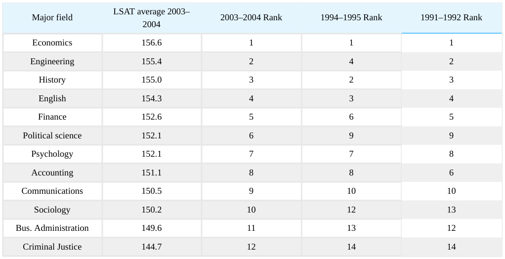
- Data from 1991 to 2004 consistently shows that economics majors achieve the highest average LSAT scores among all major undergraduate fields.
- The success of economics students is likely a combination of the field attracting naturally analytical minds and the curriculum further developing those traits.
- Beyond law, an economics background serves as a foundation for high-level research positions and competitive roles in business and industry.
- Economics and finance graduates command strong starting salaries, averaging over $45,000 as of 2006, with steady projected job growth.
- The major qualifies individuals for diverse specialized roles including actuaries, financial analysts, urban planners, and underwriters.
In rankings for all three years, economics majors recorded the highest scores.
Economics and Career Prospects
- A statistical comparison of undergraduate majors shows significant variance in starting salaries and projected job growth across disciplines.
- While earnings are a factor, the text emphasizes that major selection is also driven by personal interests, abilities, and the pursuit of satisfaction.
- The concept of opportunity cost is central to the decision-making process when choosing a field of study like economics.
- Economics is defined by three core assumptions: the consideration of opportunity costs, the maximization of self-interest, and marginal decision-making.
- The field is fundamentally divided into two primary branches: microeconomics and macroeconomics.
What is your opportunity cost of pursuing study of economics? Does studying more economics serve your interests and will doing so maximize your satisfaction level?
The Financial Payoff of Economics
- Economics majors consistently earn higher salaries than graduates in most other fields, including business administration and natural sciences.
- The financial advantage of an economics degree persists even for those who pursue graduate studies like an MBA or a law degree.
- Data suggests economics majors outperform all other common pre-law majors in terms of post-graduation wages.
- While some attribute high earnings to student intelligence, the fact that economics majors outearn physics majors suggests the specific 'economic way of thinking' is what the market rewards.
- Economics graduates are highly versatile, finding employment across a wide range of occupations, particularly in management positions.
This finding lends some credence to the notion that the marketplace rewards training in the economic way of thinking.
Microeconomics and Opportunity Cost
- The cost of raising a child involves both direct expenditures and the economic concept of opportunity cost.
- Standard estimates include housing, food, and education but often omit the value of time spent on childcare.
- Long-term financial planning must account for extended support of adult children over the age of 21.
- Microeconomic analysis specifically examines these types of individual household choices and trade-offs.
- The field of economics relies on the 'ceteris paribus' assumption to isolate variables when testing hypotheses.
- Economists distinguish between positive statements of fact and normative statements of value.
An economist would add the value of the best alternative use of the additional time that will be required for the child.
The Scientific Method in Economics
- Economics is distinguished by its focus on opportunity cost, self-interest maximization, and marginal analysis.
- The scientific method serves as a systematic framework for creating knowledge through the testing of falsifiable hypotheses.
- A hypothesis must be an assertion of a relationship between variables that is capable of being proven false through testing.
- Hypotheses that survive rigorous, widespread testing and gain general acceptance evolve into theories and eventually laws.
- Scientific laws represent high levels of confidence but can never be considered definitively proven true, as new evidence may always emerge.
There is always a possibility that someone may find a case that invalidates the hypothesis. That possibility means that nothing in economics, or in any other social science, or in any science, can ever be p r o v e n true.
Economic Models and Hypotheses
- Scientific thought relies on models which are deliberate simplifications of a reality too complex for the human mind to process.
- Economic models use intentionally false assumptions, such as an economy producing only two goods, to improve conceptual understanding.
- Graphs serve as a primary tool for economists to represent these theoretical models and generate testable hypotheses.
- Testing economic hypotheses requires empirical data, but raw observations can often appear to contradict theoretical predictions.
- The 'ceteris paribus' assumption is critical because it isolates the relationship between two variables by assuming all other factors remain unchanged.
- Apparent contradictions in data, such as rising gas prices alongside rising consumption, often stem from multiple variables shifting simultaneously.
A model of the real world cannot b e the real world.
Economic Causality and Challenges
- Economic analysis is complicated by the fact that multiple variables, such as income and population, often change simultaneously.
- Unlike laboratory sciences, economics operates in the real world where controlled experiments are rarely possible.
- The fallacy of false cause occurs when researchers incorrectly assume one variable causes another simply because they move together.
- Economists use complex statistical methods to isolate the impact of single events, though absolute certainty remains elusive.
- Despite the inability to prove causation definitively, theoretical frameworks and extensive testing provide high confidence in economic propositions.
We cannot ask the world to stand still while we conduct experiments in economic phenomena.
Positive and Normative Economics
- Positive statements are assertions of fact or hypotheses that can be tested and potentially proven false through investigation.
- Normative statements are based on value judgments and opinions, making them impossible to prove or disprove through scientific testing.
- Disagreements in economics often persist because they are rooted in differing personal values rather than conflicting data.
- The scientific method in economics is limited by the inability to prove a hypothesis true; researchers can only fail to prove it false.
- Correlation does not equal causation, as seen in the 'fallacy of false cause' where an underlying factor may drive two seemingly related conditions.
Because no test exists for these values, these two economists will continue to disagree, unless one persuades the other to adopt a different set of values.
The Economists' Tool Kit
- Scarcity forces choices because selecting one alternative necessitates giving up another, creating an opportunity cost.
- Economics is defined by its focus on opportunity costs, maximizing behavior, and marginal analysis.
- Microeconomics examines individual and market-level choices, while macroeconomics analyzes aggregate outcomes like employment and inflation.
- The scientific method in economics relies on testing hypotheses that can be refuted but never definitively proven.
- Models simplify real-world complexity through assumptions to generate testable hypotheses about economic behavior.
- Positive statements are testable facts or hypotheses, whereas normative statements are untestable value judgments.
The data are consistent with the hypothesis, but it is never possible to prove that a hypothesis is correct.
Economic Principles and Scarcity
- The text presents exercises to distinguish between normative statements, which express values, and positive statements, which describe factual relationships.
- It explores the fundamental concept of scarcity by questioning if doubling the hours in a day would eliminate the time constraint on human activity.
- Opportunity cost is examined through the lens of higher education, specifically why younger individuals are more likely to pursue degrees than older ones.
- The material addresses the 'fallacy of false cause' and the 'ceteris paribus' problem when testing economic and scientific hypotheses.
- It discusses the validity of using idealized models, such as a perfect vacuum in physics, despite their reliance on technically incorrect assumptions.
- The section introduces the 'Production Possibilities Model' as a framework for understanding how societies make choices under conditions of scarcity.
What if the quantity of time were increased, say to 48 hours per day, and everyone still lived as many days as before. Would time still be scarce?
The Factors of Production
- The three primary factors of production—labor, capital, and natural resources—are the essential building blocks used to create goods and services.
- The ultimate goal of utilizing these resources is to create utility, which is the value or satisfaction people derive from consumption.
- Labor encompasses both physical human effort and human capital, which consists of the skills gained through education and experience.
- Capital is defined specifically as a factor of production that has itself been produced for the purpose of creating other goods and services.
- The total labor capacity of an economy can be expanded by either increasing the number of workers or enhancing their human capital through training.
- Technology and entrepreneurs serve as the catalysts that organize and put these fundamental factors of production to work.
Ultimately, then, an economy’s factors of production create utility; they serve the interests of people.
Defining Capital and Natural Resources
- Capital is defined as any produced resource used to create other goods and services, ranging from ancient stone tools to modern software and symphonies.
- A critical distinction is made between physical or intellectual capital and financial capital; money itself is not capital because it cannot directly produce goods.
- Natural resources must exist in nature without human alteration and require human knowledge to be transformed into productive assets.
- The status of a substance as a resource is fluid, as seen with oil, which was once a nuisance until technological refinement gave it utility.
- Natural resources include aesthetic and environmental value, such as wilderness areas that provide utility through beauty rather than raw materials.
- The availability of natural resources can be expanded through new discoveries, new applications for existing materials, or improved extraction methods.
Pennsylvania farmers in the eighteenth century who found oil oozing up through their soil were dismayed, not delighted.
Drivers of Economic Production
- Technology and entrepreneurship are the primary forces that organize factors of production to create goods and services.
- Entrepreneurs in market economies drive innovation by seeking profit through the reorganization of resources.
- In non-market economies, bureaucrats fulfill the entrepreneurial role but respond to incentives other than profit.
- The continuous introduction of new technologies by entrepreneurs fundamentally alters how labor is performed across all sectors.
- Factors of production are categorized into labor, capital, and natural resources, with human capital being a key variable in labor quality.
We can dispute whether all the changes have made our lives better. What we cannot dispute is that they have made our lives different.
Technology and Economic Productivity
- Advanced mapping and drilling technologies have reduced the cost of discovering oil from $20 to under $5 per barrel.
- Logistics technology, such as handheld inventory computers, allows companies like PepsiCo to optimize delivery routes and reduce fleet requirements.
- In the dairy industry, electronic milkers and computer monitoring have increased milk output per cow by 50% over two decades.
- Technological progress generally benefits consumers through lower prices and workers through higher wages linked to productivity.
- While technology drives overall economic growth and profit, it also leads to job displacement and the obsolescence of certain firms.
- The Mars oil platform exemplifies the scale of modern engineering, standing 300 feet above water with tendons reaching 3,000 feet deep.
The name Mars reflects its otherworld appearance—it extends 300 feet above the water’s surface and has steel tendons that reach 3,000 feet to the floor of the gulf.
Defining Capital and Production Possibilities
- Distinguishes between natural resources and capital by highlighting that human intervention or extraction transforms raw materials into capital.
- Identifies diverse examples of capital ranging from campus libraries and power plants to the White House and national park facilities.
- Introduces the production possibilities curve as a graphical tool to represent the trade-offs between two specific goods or services.
- Explains that the model assumes fixed technology and a limited quantity of factors of production to illustrate scarcity.
- Outlines how the model differentiates between full employment of resources and inefficient, idle factors of production.
- Connects the concepts of specialization and comparative advantage to the physical constraints of the production possibilities curve.
An untapped deposit of natural gas is a natural resource. Once extracted and put in a storage tank, natural gas is capital.
Alpine Sports Production Possibilities
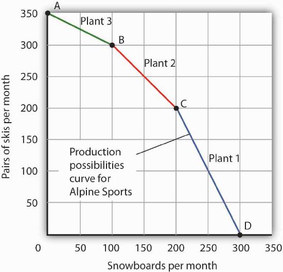
- Alpine Sports serves as a model for understanding production trade-offs between two goods: skis and snowboards.
- The firm operates three distinct plants, each with different capacities and specialized designs for production.
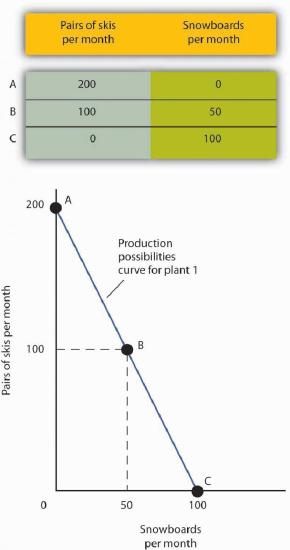
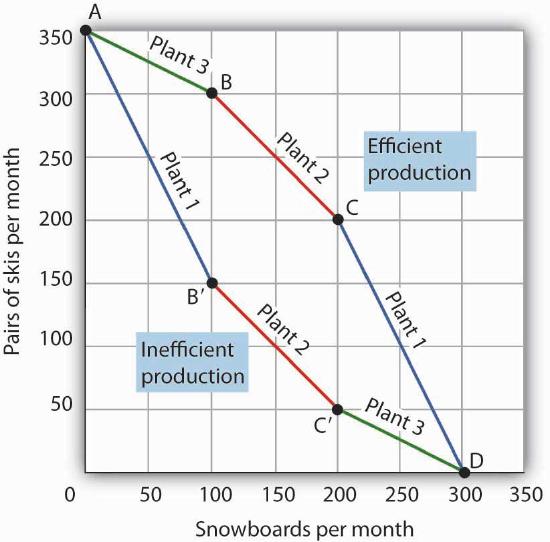
- A production possibilities curve (PPC) illustrates the maximum output combinations given fixed resources and technology.
- The downward-sloping linear curve demonstrates a negative relationship, where increasing one product necessitates decreasing the other.
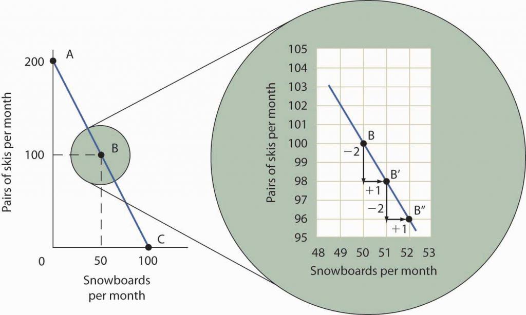
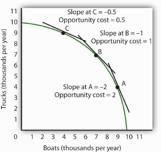
- The slope of the PPC represents the opportunity cost, specifically the rate at which one good must be sacrificed to produce another.
- Constant opportunity cost is shown through a straight-line PPC, where the trade-off ratio remains identical at all points on the curve.
The negative slope of the production possibilities curve reflects the scarcity of the plant’s capital and labor.
Opportunity Cost and Slope
- The absolute value of the slope of a production possibilities curve (PPC) represents the opportunity cost of producing one additional unit of the good on the horizontal axis.
- In a linear PPC, the slope remains constant, meaning the trade-off ratio between two goods like skis and snowboards does not change regardless of production volume.
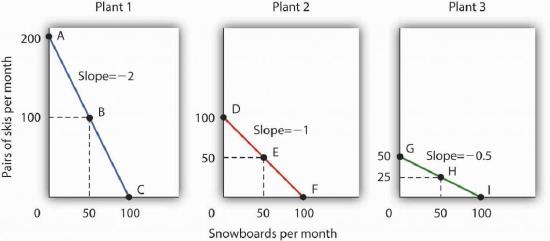
- Different production facilities often have different slopes, reflecting varying levels of efficiency and resource allocation for specific products.
- The steepness of the PPC curve is a direct visual indicator of cost; a steeper curve signifies a higher opportunity cost for the good on the horizontal axis.
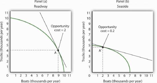
- Comparative advantage is identified by finding the plant or resource with the lowest opportunity cost, such as Plant 3 requiring only half a pair of skis per snowboard.
- To increase production of one good, resources must be freed up by reducing the production of another, a fundamental constraint of the PPC model.
The greater the absolute value of the slope of the production possibilities curve, the greater the opportunity cost will be.
Comparative Advantage and Production Curves
- A combined production possibilities curve is constructed by aggregating the maximum output capacities of multiple individual plants.
- When shifting production from one good to another, efficient firms prioritize plants with the lowest opportunity cost for the new product.
- Comparative advantage is defined as the ability to produce a good at a lower opportunity cost than other entities.
- A plant can possess a comparative advantage not through superior proficiency, but through a lack of efficiency in producing alternative goods.
- The sequence of shifting production across plants creates a bowed-out combined curve, reflecting increasing opportunity costs as more resources are diverted.
Comparative advantage thus can stem from a lack of efficiency in the production of an alternative good rather than a special proficiency in the production of the first good.
The Law of Increasing Opportunity Cost
- The production possibilities curve is constructed from linear segments representing individual assembly plants.
- The resulting curve exhibits a bowed-out shape rather than a straight line.
- The absolute value of the curve's slope increases as production shifts toward a single good.
- This shape is a direct consequence of allocating resources based on the principle of comparative advantage.
- The transition from skis to snowboards illustrates how opportunity costs change with production volume.
Notice that this production possibilities curve, which is made up of linear segments from each assembly plant, has a bowed-out shape; the absolute value of its slope increases as Alpine Sports produces more and more snowboards.
Law of Increasing Opportunity Cost
- The law of increasing opportunity cost states that as production of a specific good rises, the cost of producing additional units in terms of sacrificed alternatives also increases.
- This economic principle is visually represented by a bowed-out or concave production possibilities curve rather than a straight line.
- The curve's shape is driven by comparative advantage, as resources (like different manufacturing plants) are not equally efficient at producing all goods.
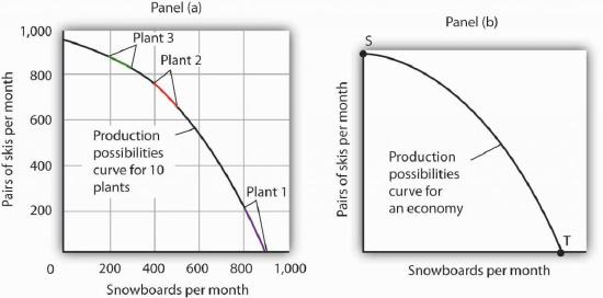
- As more production units or plants are added to a model, the production possibilities curve transitions from jagged segments into a smooth, continuous curve.
- In large-scale economies with millions of participants, economists typically use smooth, numberless curves to illustrate general production trade-offs and scarcity.
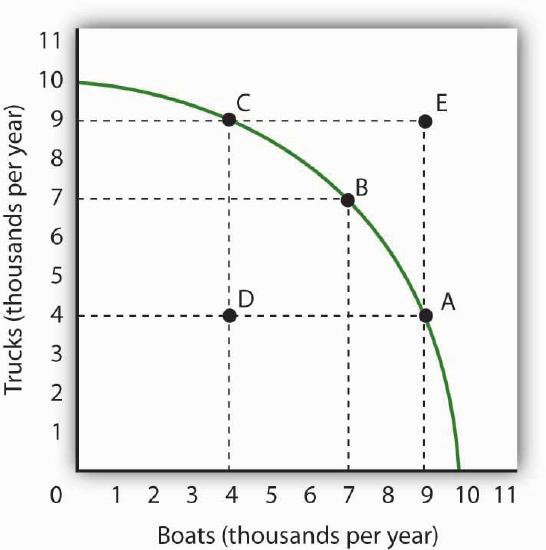
Scarcity implies that a production possibilities curve is downward sloping; the law of increasing opportunity cost implies that it will be bowed out, or concave, in shape.
The Production Possibilities Model
- Economic models often assume production curves are smooth and 'bowed out' to represent trade-offs.
- The model simplifies reality by focusing on an economy that produces only two specific goods.
- A core assumption is that technology and available factors of production remain constant during the analysis.
- Operating on the curve implies that increasing one good's production requires reducing the other.
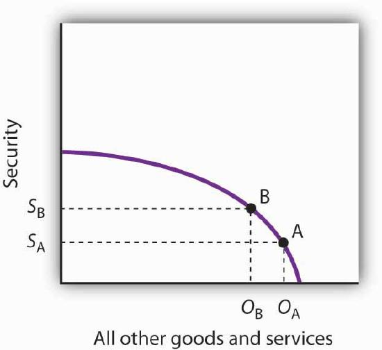
- The model can be applied to macro-level choices, such as balancing national security against all other goods.
In this section, we shall assume that the economy operates on its production possibilities curve so that an increase in the production of one good in the model implies a reduction in the production of the other.
The Cost of Security
- National security is treated as a category of production that competes with all other goods and services for limited resources.
- The shift toward increased security spending after 9/11 illustrates a movement along the production possibilities curve.
- Increasing security requires tangible resources, such as personnel for airport inspections and state-level counter-terrorism efforts.
- The law of increasing opportunity cost suggests that as more security is produced, the sacrifice of other goods becomes progressively larger.
- The production possibilities model identifies the trade-offs available to a nation but does not dictate which specific point on the curve is optimal.
Of course, an economy cannot really produce security; it can only attempt to provide it.
Inside the Production Curve
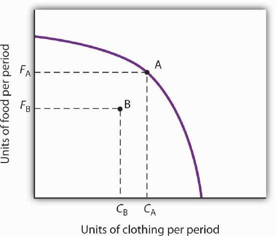
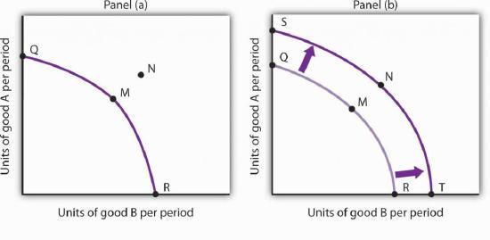
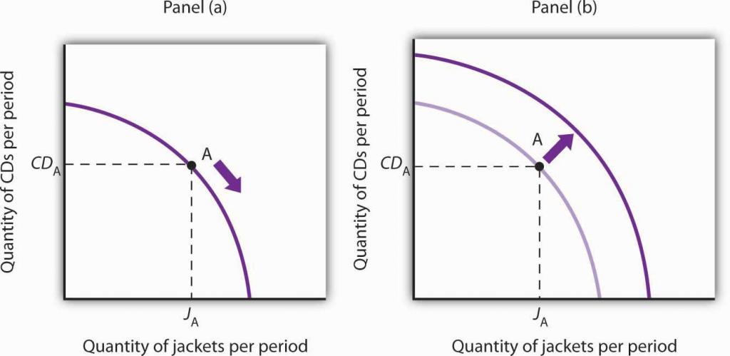
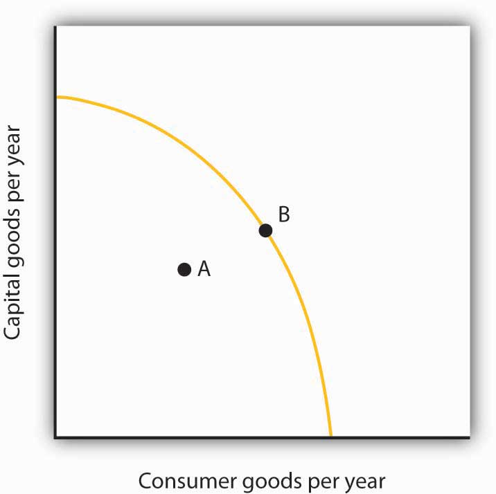
- Operating inside the production possibilities curve indicates an economy is failing to maximize its potential output of goods and services.
- The failure to achieve full employment of labor, buildings, or land results in a level of production that falls short of the curve.
- Beyond unemployment, an economy can underperform if it fails to allocate its resources based on the principle of comparative advantage.
- Moving from inside the curve to the boundary allows an economy to increase the production of all goods simultaneously, raising the standard of living.
- The production possibilities model highlights that job loss is not just a loss of income for workers, but a loss of tangible goods for the entire society.
Some workers are without jobs, some buildings are without occupants, some fields are without crops.
Efficiency and Comparative Advantage
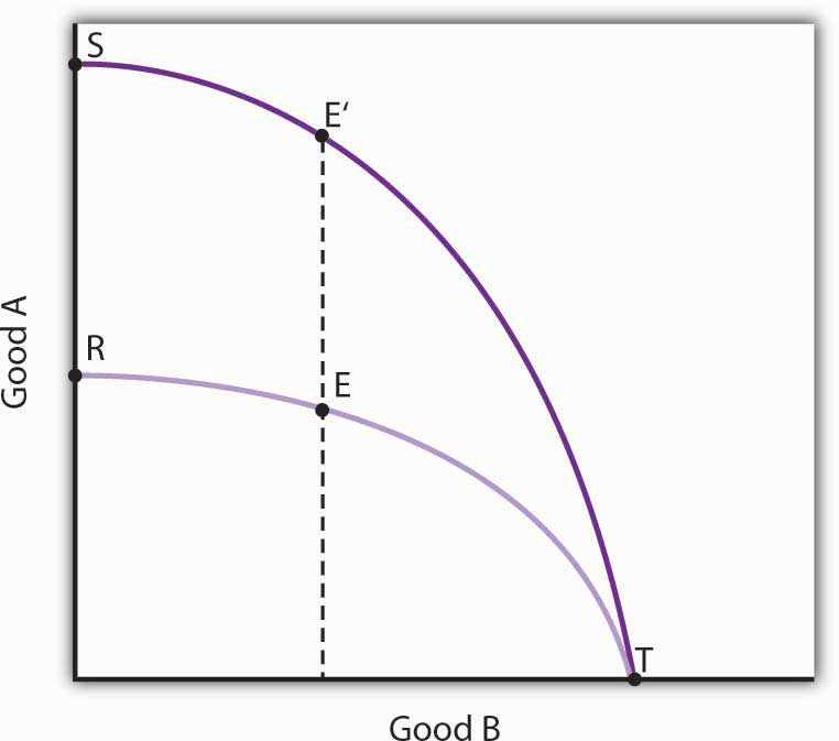
- Allocating resources without considering comparative advantage results in a bowed-in production curve rather than a bowed-out one.
- Inefficient production occurs when an economy operates inside its production possibilities curve, producing fewer goods than its resources allow.
- By switching production based on comparative advantage, a firm can increase the output of all goods simultaneously without adding more labor or capital.
- Efficient production requires both the full use of available factors and the optimal allocation of those factors.
- The production possibilities curve serves as a guide for how goods should be produced to maximize societal output.
Inefficient production implies that the economy could be producing more goods without using any additional labor, capital, or natural resources.
Specialization and Comparative Advantage
- Specialization occurs when an economy produces goods and services in which it holds a comparative advantage.
- Individual workers specialize in specific fields and use their income to trade for goods produced by others with different advantages.
- The absence of specialization would lead to a drastic decline in living standards, making survival difficult for most people.
- Nations allocate resources based on land and population endowments, such as the U.S. focusing on agriculture while Hong Kong focuses on nonagricultural uses.
- The production possibilities curve is bowed outward because resources are allocated according to the law of increasing opportunity cost.
- Operating inside the production possibilities curve indicates an inefficient use of an economy's factors of production.
Imagine that you are suddenly completely cut off from the rest of the economy. You must produce everything you consume; you obtain nothing from anyone else.
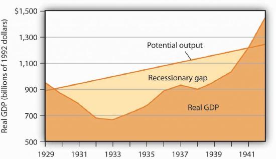
Costs of the Great Depression
- The U.S. economy transitioned from unprecedented prosperity in early 1929 to a severe contraction that left resources vastly underutilized.
- By 1933, unemployment exceeded 25% and national production had plummeted by nearly 30%, moving the economy far inside its production possibilities curve.
- Full employment of resources was not achieved again until 1942, driven by the massive mobilization required for World War II.
- The cumulative loss of goods and services between 1929 and 1942 is estimated at over $3 trillion in modern currency.
- The material cost of the output lost during the Great Depression actually exceeded the total financial cost of fighting World War II.
- The production possibilities model serves as a framework for understanding international trade, economic growth, and the efficiency of different economic systems.
In material terms, the forgone output represented a greater cost than the United States would ultimately spend in World War II.
Comparative Advantage in Trade
- Nations function like individual production plants, each possessing a unique comparative advantage in specific activities.
- Global efficiency is maximized when nations specialize in goods where they hold a comparative advantage rather than attempting self-sufficiency.
- Specialization creates a state of mutual interdependence where nations must trade their surplus for goods produced more efficiently elsewhere.
- A refusal to trade results in world production falling inside the production possibilities curve, indicating a waste of potential resources.
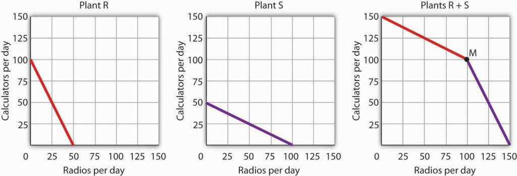
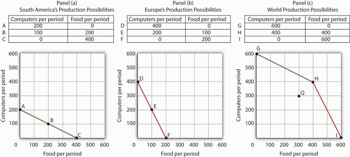
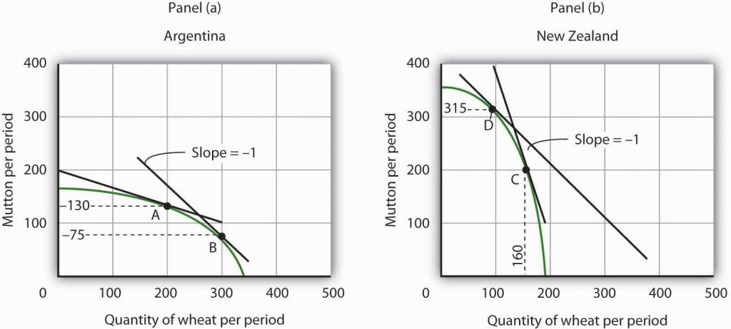
- Using a model of South America and Europe, the text demonstrates that free trade allows for a higher total output of both food and computers.
A failure to allocate resources in this way means that world production falls inside the production possibilities curve; more of each good could be produced by relying on comparative advantage.
The Power of Comparative Advantage
- The world production possibilities curve takes on a bowed-out shape even when individual nations have linear curves.
- Specialization based on comparative advantage allows for a higher total output of goods without requiring additional resources.
- Trade restrictions force the world to operate inside its production possibilities curve, resulting in lower overall production.
- A nation's trade policy affects the distribution of employment across sectors but does not dictate the overall level of employment.
- While trade creates enormous global benefits, it necessitates the reallocation of resources which can incur transition costs.
- Economists generally agree that free trade is desirable as it promotes greater production of goods and services for the global population.
Of course, this idealized example would have all of South America’s computer experts becoming farmers while all of Europe’s farmers become computer geeks!
Mechanics of Economic Growth
- Economic growth is defined as an outward shift in a production possibilities curve, making previously unattainable production levels possible.
- Growth is driven by increases in the physical quantity or quality of factors of production, such as labor and capital.
- Technological gains, ranging from automated production to advanced information technology, significantly reduce the time and effort required for output.
- Human capital has seen dramatic improvements, evidenced by U.S. high school completion rates rising from 3.5% in 1900 to 92% in 2006.
- Modern innovations like computer-based oil mapping and automated milking demonstrate how technology fuels growth across diverse sectors.
The development of modern information technology—including computers, software, and communications equipment—that seemed to proceed at breathtaking pace especially during the final years of the last century and continuing to the present has transformed the way we live and work.
Sources of Economic Growth
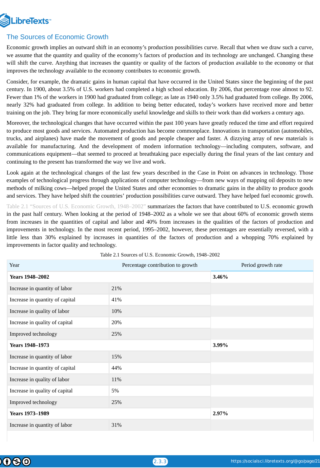
- U.S. economic growth shifted from being driven by factor quantities to being driven by factor quality and technology.
- Between 1948 and 2002, total economic output increased sixfold, with technology and capital quality playing increasingly dominant roles.
- In the 1995-2002 period, improvements in technology and capital quality accounted for a 'whopping' 70% of growth.
- The surge in growth during the late 1990s is largely attributed to the rapid integration of information technology in the workplace.
- The contribution of capital quantity significantly dropped in the most recent period, falling to just 8% compared to historical highs of 44%.
In the most recent period, 1995–2002, however, these percentages are essentially reversed, with a little less than 30% explained by increases in quantities of the factors of production and a whopping 70% explained by improvements in factor quality and technology.
Sacrifice for Future Growth
- Economic growth requires the postponement of current consumption to invest in future productive capability.
- Capital formation, such as the creation of tools or infrastructure, is a primary result of delaying immediate gratification.
- Human capital is developed through personal sacrifices, such as students choosing study over immediate income-earning work.
- A society's production possibilities curve shifts outward when resources are diverted from consumer goods to capital goods.
- The incentive to achieve production efficiency is often driven by the pursuit of profit within specific economic systems.
When Stone Age people fashioned the first tools, they were spending time building capital rather than engaging in consumption.
The Spectrum of Economic Systems
- Global economies exist on a spectrum ranging from market capitalism to command socialism.
- Market capitalism is characterized by private ownership and individual decision-making regarding resource use.
- Command socialism involves government ownership of capital and natural resources with centralized allocation power.
- Mixed economies incorporate varying elements of both capitalist and socialist systems.
- No real-world economy functions as a pure case of either extreme; they are evaluated by the degree of government intervention.
- Countries like the United States and Chile represent the capitalist end, while North Korea and Cuba represent the socialist end.
No economy represents a pure case of either market capitalism or command socialism.
The Spectrum of Economic Systems
- Economies exist on a spectrum ranging from command socialist to market capitalist, with many nations like France and Germany operating in the regulated center.
- The global shift toward market capitalism in the late 20th century was driven by its emphasis on individual freedom and decision-making power.
- Market-based systems tend to allocate resources more efficiently by leveraging comparative advantage, leading to higher production levels.
- Entrepreneurial activity is most robust in market capitalist systems where individuals can profit directly from the efficient use of resources.
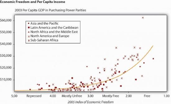
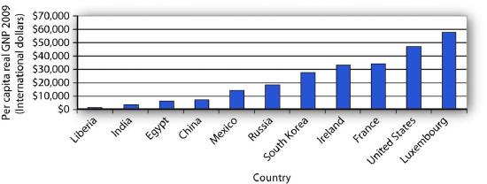
- Data from the Heritage Foundation suggests a strong positive correlation between a nation's degree of economic freedom and its per capita income.
- Heavy government regulation or state ownership can stifle productivity by prohibiting the flexible transfer of resources between different uses.
If she were operating under a command socialist system, she would not be the owner of the plants and thus would be unlikely to profit from their efficient use.
Economic Freedom and Government Roles
- Market capitalist economies are defined and measured by the degree of economic freedom they permit.
- Data from the Heritage Foundation suggests a strong correlation between high economic freedom and higher per capita income.
- While correlation exists, economists must avoid the fallacy of false cause when linking freedom to income growth.
- Governments in market economies influence production through taxes, subsidies, and the prohibition of certain goods.
- Public agencies act as the primary providers for essential services like national defense and law enforcement where private markets may not exist.
North Korea received the dubious distinction of being the least free.
Economic Growth and European Integration
- Comparative advantage and specialization are identified as primary drivers for increasing the production of goods and services through international trade.
- Economic growth requires increasing the quantity or quality of factors of production, often necessitating a postponement of current consumption to build capital.
- Market capitalist systems are noted for generally outperforming mixed or command socialist economies in terms of overall productivity.
- The European Union serves as a major real-world application of comparative advantage by eliminating trade barriers and establishing a common currency.
- The origins of European integration were radical and revolutionary, beginning with a 1950 proposal for steel cooperation between former enemies France and Germany.
The proposal for cooperation between two countries that had been the most bitter of enemies was a revolutionary one.
European Union Comparative Advantage
- The European Union functions similarly to the United States by dismantling internal trade restrictions and ceding national sovereignty to a central entity.
- Removing trade barriers allowed member nations to move from inside their collective production possibilities curve to a more efficient frontier.
- Research indicates that expanded trade within the EU is primarily driven by specialization based on comparative advantage within specific industries.
- Northern European nations like Germany and France specialize in high-value goods such as technology and luxury automobiles.
- Southern European nations like Spain and Portugal specialize in lower-value goods, including textiles, food, and budget-friendly vehicles.
- Specialization across the Union corresponds to national income levels and human capital, ultimately increasing the welfare of all member citizens.
Just as the U.S. Constitution prohibits states from restricting trade with other states, the European Union has dismantled all forms of restrictions that countries within the Union used to impose on one another.
The Production Possibilities Model
- Economics centers on the allocation of labor, capital, and natural resources through specific production choices.
- The production possibilities curve is downward sloping and bowed out, illustrating scarcity and the law of increasing opportunity cost.
- Comparative advantage drives efficient production choices and forms the theoretical basis for the benefits of international trade.
- Economic growth is achieved by increasing the quantity or quality of factors of production or through technological advancement.
- Economic systems are defined by the ownership of resources, with a global trend moving toward market capitalist models for higher productivity.
- While market systems are favored, government remains essential for establishing legal frameworks and providing social safety nets.
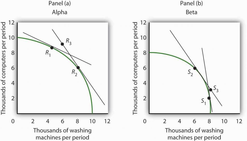
Producing each additional unit of the good on the horizontal axis requires a greater sacrifice of the good on the vertical axis than did the previous units produced.
Production Possibilities and Trade
- The text explores how technological improvements in one sector shift the production possibilities curve and alter opportunity costs.
- It examines the impact of resource restrictions, such as labor bans or trade barriers, on a nation's total economic output.
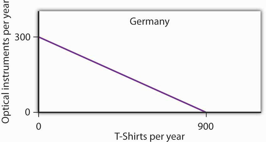
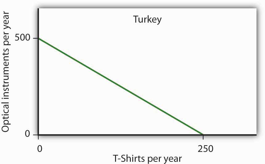
- The concept of comparative advantage is tested through scenarios involving specialized resources in different countries.
- The relationship between investment and consumption is questioned to determine if prioritizing growth is always a desirable social choice.
- Numerical problems are used to calculate opportunity costs and slopes to identify comparative advantages between individuals and nations.
Suppose blue-eyed people were banned from working. How would this affect a nation’s production possibilities curve?
Principles of Demand and Supply
- The text transitions from comparative advantage exercises involving Turkey and Germany to the fundamental principles of demand and supply.
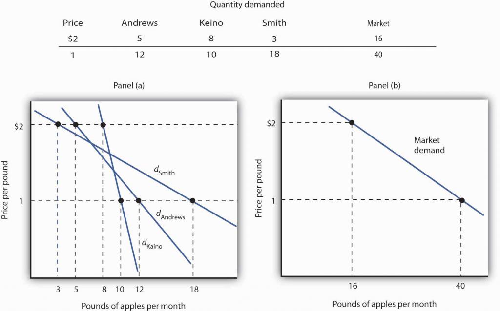
- Quantity demanded is defined as the specific amount of a good or service consumers are willing and able to purchase at various price points.
- Economists distinguish between a movement along a demand curve, caused by price changes, and a shift in the curve, caused by external variables.
- Key determinants of demand beyond price include consumer preferences, income levels, demographic characteristics, and the prices of related goods.
- The law of demand is illustrated by the inverse relationship between price and quantity, where higher prices typically reduce consumer desire for a product.
How many pizzas will people eat this year? How many doctor visits will people make? How many houses will people buy?
Defining Demand and Quantity
- Economists distinguish between 'demand' as a general concept and 'quantity demanded,' which refers to a specific amount at a specific price.
- The 'ceteris paribus' assumption is essential to isolating the relationship between price and quantity by holding all other variables constant.
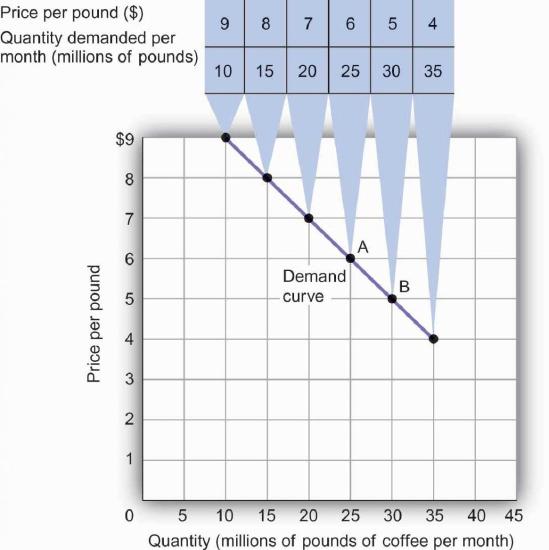
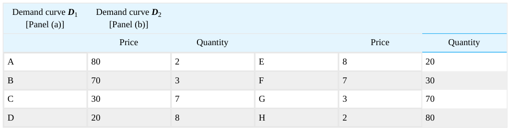
- A demand schedule provides a tabular view of how different price points correlate with the quantities buyers are willing to purchase.
- A demand curve serves as a graphical representation of the schedule, typically plotting price on the vertical axis and quantity on the horizontal axis.
- Movement along the demand curve is strictly defined as a 'change in quantity demanded' resulting from a change in price alone.
The quantity demanded of a good or service is the quantity buyers are willing and able to buy at a particular price during a particular period, all other things unchanged.
The Law of Demand
- The law of demand establishes a fundamental behavioral relationship where price and quantity demanded move in opposite directions.
- A movement along the demand curve occurs when the price of a good changes while all other factors remain constant.
- Empirical evidence from numerous economic studies consistently supports the validity of the law of demand.
- Retailers practically apply this law by lowering prices during sales to clear overstock and increase consumer purchases.
- The negative slope of the demand curve is a visual representation of the inverse relationship between price and quantity.
When a store finds itself with an overstock of some item, such as running shoes or tomatoes, and needs to sell these items quickly, what does it do?
Shifts in the Demand Curve
- While price influences consumption, other variables like income, population, and preferences also dictate the quantity of goods demanded.
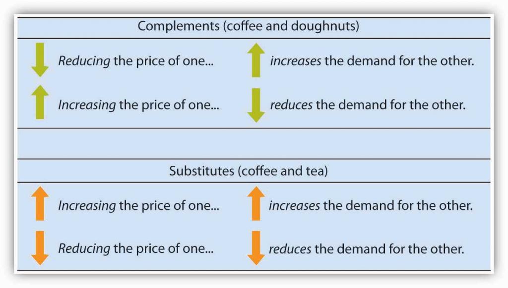
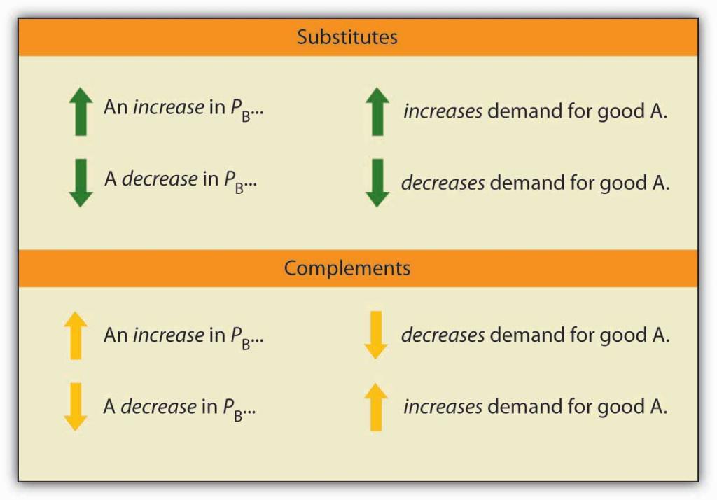
- The prices of related goods, such as complements like doughnuts or substitutes like tea, significantly impact the demand for a specific product.
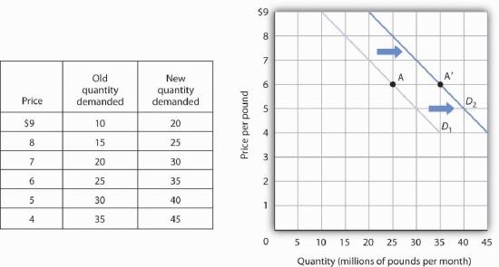
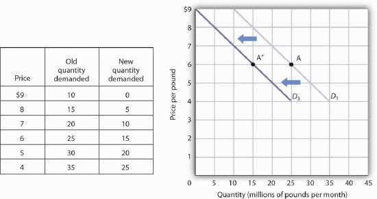
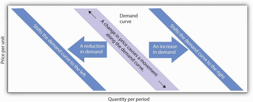
- A change in any variable held constant during the creation of a demand schedule results in a shift of the entire demand curve rather than a movement along it.
- An increase in demand is represented graphically as a rightward shift, meaning more of a product is purchased at every given price point.
- A decrease in demand, or a leftward shift, can be triggered by external factors such as negative health findings or a reduction in the consumer population.
- Economists distinguish between a 'change in quantity demanded' (movement along the curve) and a 'change in demand' (a shift of the curve itself).
A shift in a demand curve is called a change in demand.
Determinants of Market Demand
- Demand shifters include consumer preferences, prices of related goods, income levels, demographics, and buyer expectations.
- Changes in consumer preferences, such as health concerns regarding cigarettes, can shift the demand curve significantly to the left or right.
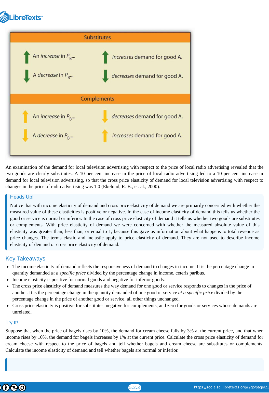
- Related goods are classified as complements, which are used together, or substitutes, which are used in place of one another.
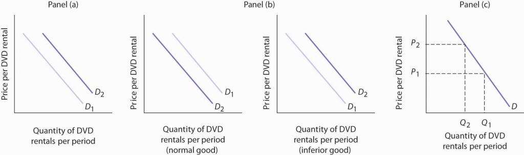
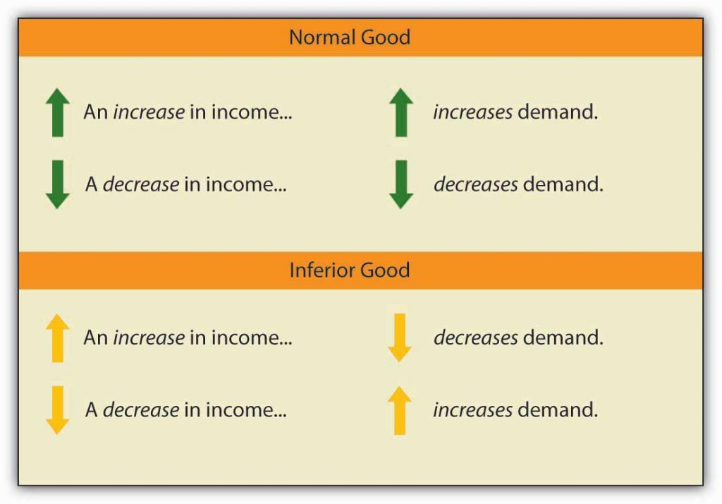
- Income levels distinguish normal goods, where demand rises with wealth, from inferior goods, where demand falls as income increases.
- Demographic shifts, such as an aging population or changes in birth rates, create long-term fluctuations in demand for specific services like healthcare or education.
A good for which demand increases when income increases is called a normal good. A good for which demand decreases when income increases is called an inferior good.
Dynamics of Buyer Demand
- Buyer expectations regarding future prices and technology significantly influence current consumption patterns for storable goods.
- Economists distinguish between a change in 'quantity demanded' (movement along a curve) and a 'change in demand' (a shift of the curve itself).
- The law of demand dictates that higher prices generally reduce the quantity demanded, provided all other factors remain unchanged.
- Demand shifters such as preferences, income, demographics, and the prices of related goods cause the entire demand curve to move.
- Goods are categorized as substitutes or complements based on how price changes in one affect the demand for the other.
- Income levels define whether a product is a 'normal good' (demand rises with income) or an 'inferior good' (demand falls with income).
If people expect gasoline prices to rise tomorrow, they will fill up their tanks today to try to beat the price increase.
Solving Campus Parking Problems
- University parking demand has surged, with 70% of students owning cars and many driving even for short five-minute commutes.
- Most universities heavily subsidize parking, losing between $400,000 and $1.2 million annually per 1,000 spaces, with costs hidden in general tuition.
- Administrators often avoid raising parking fees to market rates due to fear of political backlash from students, parents, and faculty.
- Shifting demand through substitutes, such as free carpooling and public transit, has proven more effective than expanding infrastructure.
- The University of Washington and University of Colorado saved millions by investing in commuter alternatives rather than expensive parking structures.
Indeed, according to Clark Kerr, a former president of the University of California system, a university is best understood as a group of people “held together by a common grievance over parking.”
Dynamics of Demand and Supply
- The demand for substitute goods, such as DVD rentals, increases when the price of the primary alternative, like movie tickets, rises.
- Changes in family income shift demand curves differently depending on whether a product is classified as a normal or inferior good.
- A change in a product's own price results in a movement along the demand curve rather than a shift of the curve itself.
- Quantity supplied is primarily driven by price, where higher prices typically incentivize sellers to offer more goods, assuming all other factors remain constant.
- Supply is influenced by production costs, including factor prices, technology, seller expectations, and the total number of market participants.
- External variables like natural events and weather changes can significantly impact the cost of production and the resulting supply curve.
The latter may be the case for some families, since staying at home and watching DVDs is a cheaper form of entertainment than taking the family to the movies.
The Law of Supply
- The quantity supplied is defined as the amount sellers are willing to provide at a specific price, assuming all other factors remain constant.
- The law of supply generally dictates that higher prices lead to an increase in the quantity supplied because of higher profit incentives.
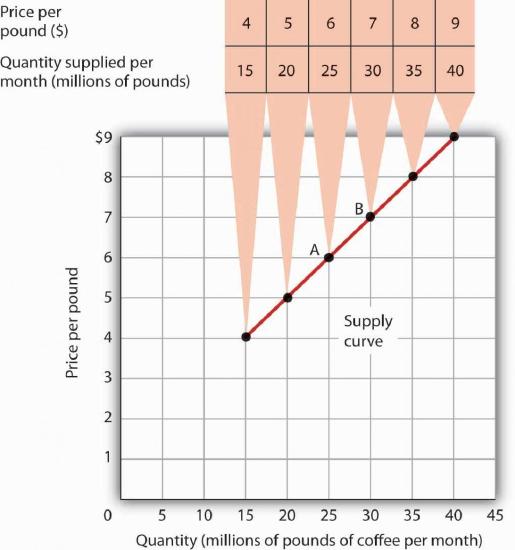
- Supply schedules and supply curves provide tabular and graphical representations of the positive relationship between price and quantity.
- Exceptions to the law of supply exist, such as fixed-supply goods like specific real estate or rare cases where higher prices reduce supply.
- A change in price results in a movement along the supply curve, which is technically termed a change in quantity supplied rather than a shift in the curve.
Goods that cannot be produced, such as additional land on the corner of Park Avenue and 56th Street in Manhattan, are fixed in supply—a higher price cannot induce an increase in the quantity supplied.
Mechanics of Supply Shifters
- Supply curves are drawn under the assumption that all variables other than price remain constant.
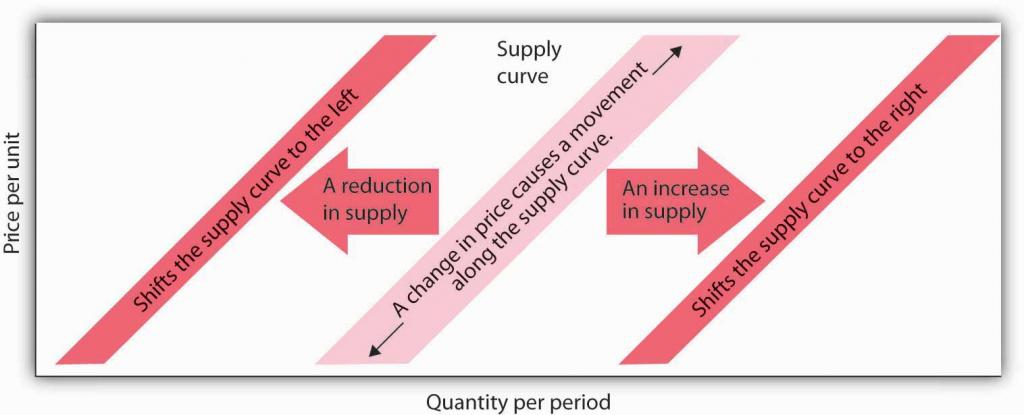
- A change in external variables results in a shift of the entire supply curve rather than a movement along it.
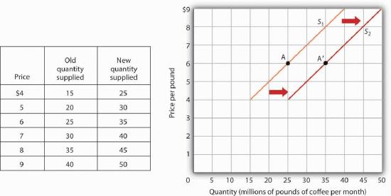
- Factors that increase supply, such as lower production costs, shift the curve to the right, increasing quantity at every price point.
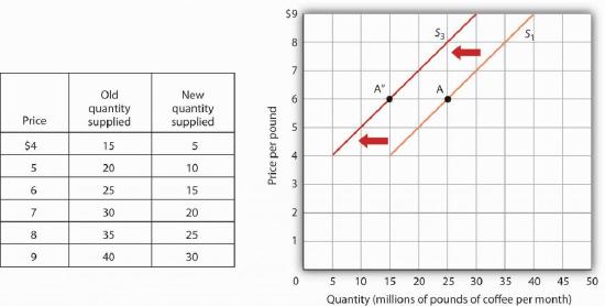
- Factors that decrease supply, such as natural disasters or rising labor costs, shift the curve to the left.
- Key supply shifters include production factor prices, technology, seller expectations, and the number of market participants.
- The cost of factors of production, like labor and fertilizer, directly dictates the quantity suppliers are willing to offer at a given price.
When these other variables change, the all-other-things-unchanged conditions behind the original supply curve no longer hold.
Factors Influencing Market Supply
- Opportunity cost dictates that producing one good requires forgoing another, meaning a price rise in a related good can decrease the supply of the current one.
- Technological advancements lower production costs and increase profit margins, shifting the supply curve to the right.
- Government regulations, such as mandatory pollution-control devices, can act as a technological reversal by increasing costs and reducing supply.
- Seller expectations regarding future price increases can lead producers to withhold current inventory, effectively shifting supply to the left.
- Natural events and disasters, such as the 2008 Myanmar cyclone, create unpredictable shifts in agricultural supply by destroying production capacity.
If a change in the international political climate leads many owners to expect that oil prices will rise in the future, they may decide to leave their oil in the ground, planning to sell it later when the price is higher.
Dynamics of Supply Curves
- The number of sellers in an industry directly impacts the supply curve, with more sellers shifting it to the right and fewer shifting it to the left.
- It is critical to distinguish between a change in supply, which shifts the entire curve, and a change in quantity supplied, which is a movement along the curve caused by price changes.
- Supply shifters include production factor prices, technology, seller expectations, natural events, and the number of market participants.
- A common student error is misinterpreting a rightward shift as a 'downward' move due to the upward slope of the supply curve.
- An increase in supply always moves toward a higher quantity on the horizontal axis, regardless of the vertical appearance of the curve.
Students sometimes make the mistake of thinking of such a shift as a shift “down” and therefore as a reduction in supply.
Monastic Opportunity Costs
- The monks of St. Benedict’s monastery transitioned through three distinct business models: egg production, cookie manufacturing, and private retreats.
- Rising grain prices in the 1970s and 1980s doubled production costs for eggs, forcing the monks to adopt more aggressive agricultural practices.
- The shift from eggs to cookies was driven by a comparative analysis of profitability and the desire for a better quality of life, specifically the ability to take Sundays off.
- Market demand influenced their decisions, as declining egg consumption due to health concerns coincided with the success of their mail-order cookie experiment.
- Ultimately, the monks moved into the retreat business because it offered the highest return on investment and required the least amount of daily labor.
- This case study illustrates the economic principle of opportunity cost, where the monks consistently chose the path that maximized both financial and spiritual resources.
“The chickens didn’t stop laying eggs on Sunday,” Father Joseph chuckles. “When we shifted to cookies we could take Sundays off. We weren’t hemmed in the way we were with the chickens.”
Supply Dynamics and Market Equilibrium
- An increase in the wages of production factors, such as rental clerks, raises production costs and shifts the supply curve to the left.
- Wage increases for specific workers should be viewed as supply shifters rather than significant drivers of consumer demand.
- Changes in the price of a good do not shift the supply curve but instead cause movement along the existing curve.
- The entry of more firms into a market increases the number of suppliers, shifting the supply curve to the right.
- The model of demand and supply combines both curves to determine the equilibrium price and quantity in a given market.
- Market imbalances, such as surpluses and shortages, create natural pressures that drive prices toward equilibrium.
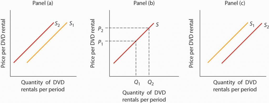
An increase in the price of DVD rentals does not shift the supply curve at all; rather, it corresponds to a movement upward to the right along the supply curve.
Market Equilibrium Dynamics
- The demand curve represents the quantity buyers are willing and able to purchase at various price points.
- The supply curve illustrates the quantities sellers are prepared to offer for sale at those same prices.
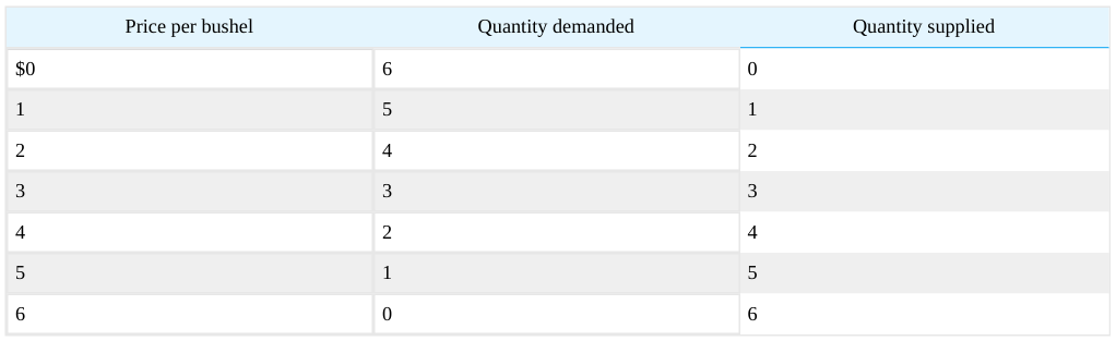
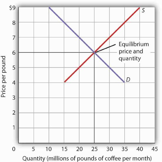
- Market equilibrium occurs at the specific intersection where the quantity demanded exactly equals the quantity supplied.
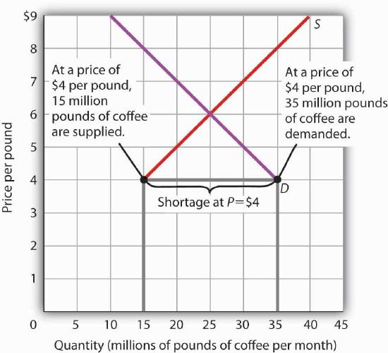
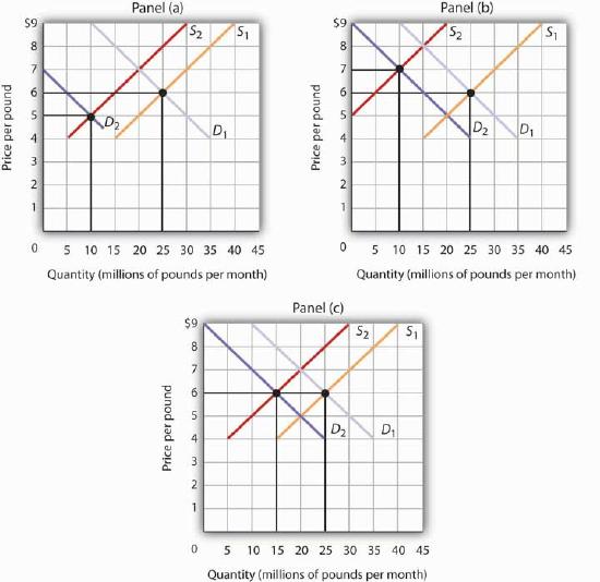
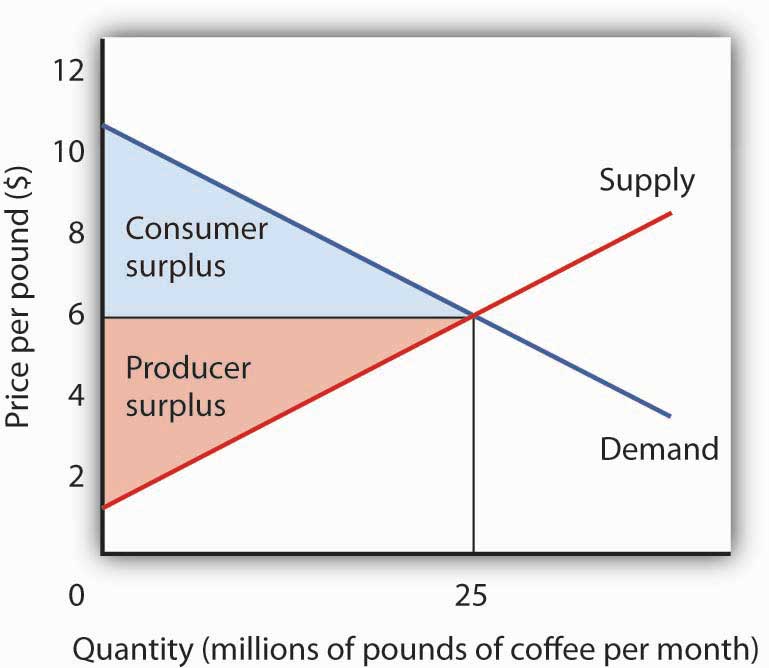
- In the provided coffee market example, equilibrium is reached at a price of $6 per pound and a quantity of 25 million pounds.
- Unless external factors cause the curves to shift, there is no inherent pressure for the equilibrium price to change.
- Any price point above or below the intersection results in a market imbalance, leading to either surpluses or shortages.
The equilibrium price in any market is the price at which quantity demanded equals quantity supplied.
Market Surpluses and Shortages
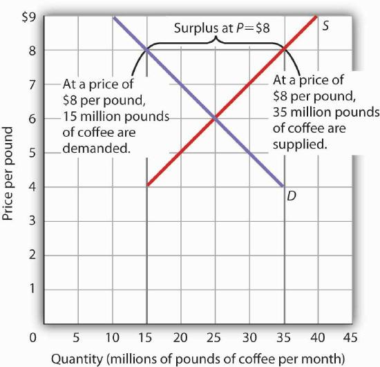
- A surplus occurs when the current market price is set above the equilibrium level, resulting in a quantity supplied that exceeds the quantity demanded.
- In response to a surplus, sellers naturally lower prices to clear unsold inventory, which simultaneously decreases supply quantity and increases demand quantity.
- A shortage arises when the market price falls below equilibrium, leading to a situation where consumers demand more than sellers are willing to provide.
- Market forces typically correct shortages as sellers raise prices, causing a movement along the curves until the equilibrium intersection is reached.
- Price adjustments serve as a self-correcting mechanism in most markets, though some specific goods may adjust to equilibrium very slowly or not at all.
With unsold coffee on the market, sellers will begin to reduce their prices to clear out unsold coffee.
Market Equilibrium and Curve Shifts
- Changes in demand or supply shifters alter the equilibrium price and quantity of a good or service.
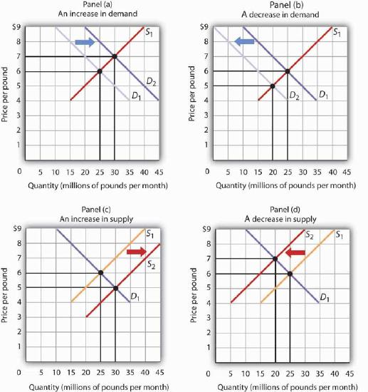
- An increase in demand shifts the demand curve right, raising both the equilibrium price and the quantity supplied.
- A decrease in demand shifts the curve left, resulting in a lower equilibrium price and a reduction in quantity supplied.
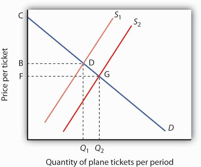
- Supply increases shift the supply curve right, which lowers the equilibrium price while increasing the quantity demanded.
- Shifts in one curve cause movement along the other curve rather than shifting both simultaneously in the initial response.
- External factors like weather, income, and the price of complements or substitutes act as the primary drivers for these shifts.
Notice that the supply curve does not shift; rather, there is a movement along the supply curve.
Supply Shifters and Market Equilibrium
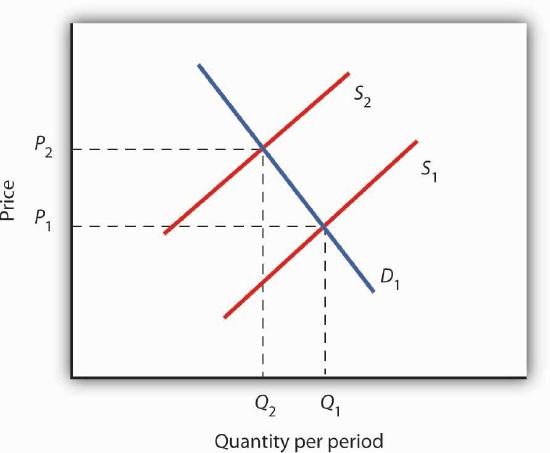
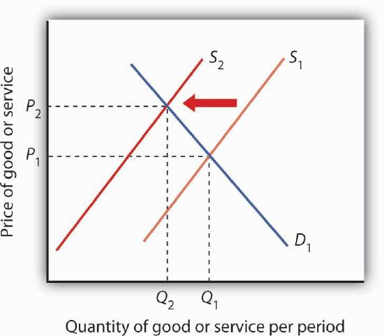
- A decrease in supply shifts the supply curve to the left, resulting in a higher equilibrium price and a lower quantity demanded.
- Factors that reduce supply include rising input costs, better returns on alternative products, technological setbacks, or natural disasters.
- When analyzing market changes, it is crucial to distinguish between a shift in the entire curve and a movement along the curve.
- A common analytical error is confusing a change in quantity demanded with a change in demand itself.
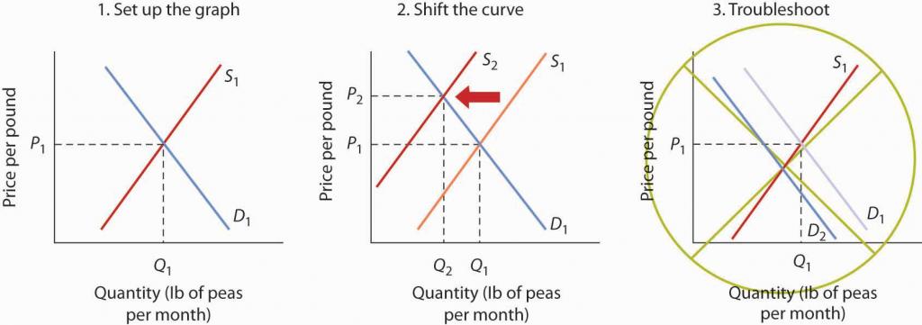
- The 'Heads Up!' section provides a step-by-step methodology for graphing supply and demand shifts using plausible numerical values.
- Logical consistency checks, such as ensuring a scarcity of goods leads to a price increase, help verify the accuracy of economic models.
Suppose you are told that an invasion of pod-crunching insects has gobbled up half the crop of fresh peas, and you are asked to use demand and supply analysis to predict what will happen to the price and quantity of peas demanded and supplied.
Simultaneous Shifts in Market Equilibrium
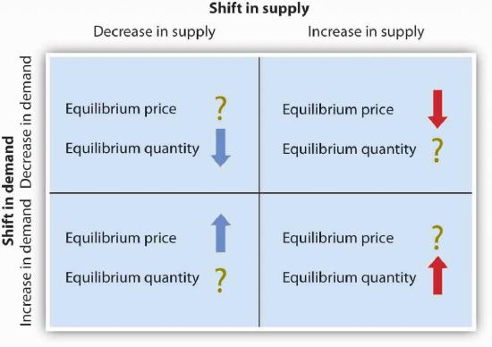
- Single shifts in demand or supply produce predictable changes in both equilibrium price and quantity.
- When both demand and supply shift simultaneously, the outcome for at least one variable becomes ambiguous.
- A simultaneous decrease in both demand and supply will always result in a lower equilibrium quantity.
- The direction of price change during simultaneous shifts depends entirely on the relative magnitude of each curve's movement.
- If demand shifts further left than supply, price falls; if supply shifts further left than demand, price rises.
- Analyzing complex market changes requires breaking down events separately to determine their individual impacts on price and quantity.
Whether the equilibrium price is higher, lower, or unchanged depends on the extent to which each curve shifts.
Market Equilibrium and Curve Dynamics
- Prices act as the primary mechanism to balance the quantity demanded with the quantity supplied.
- Without price adjustments, the essential balance between market supply and demand cannot be maintained.
- Linear representations of supply and demand curves are used as a simplification to enhance readability.
- Regardless of their shape, demand curves consistently slope downward while supply curves generally slope upward.
- Analyzing shifts in these curves allows for the prediction of changes in market price and quantity.
If prices did not adjust, this balance could not be maintained.
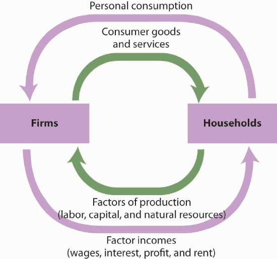
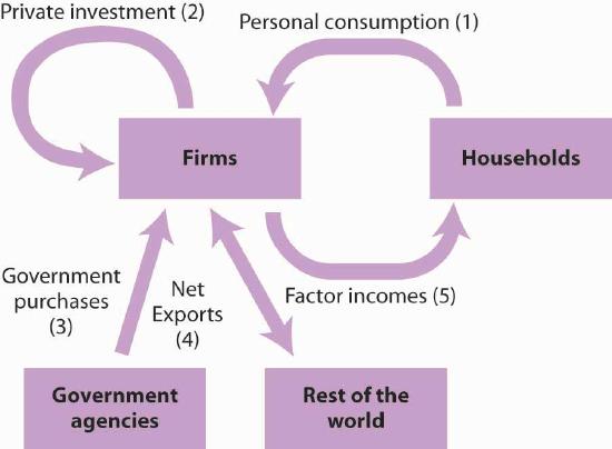
The Circular Flow Model
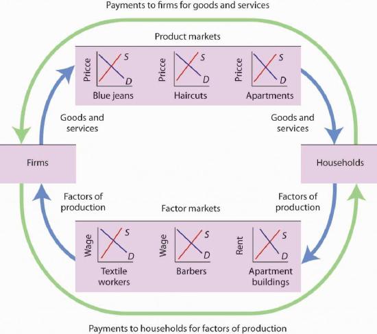
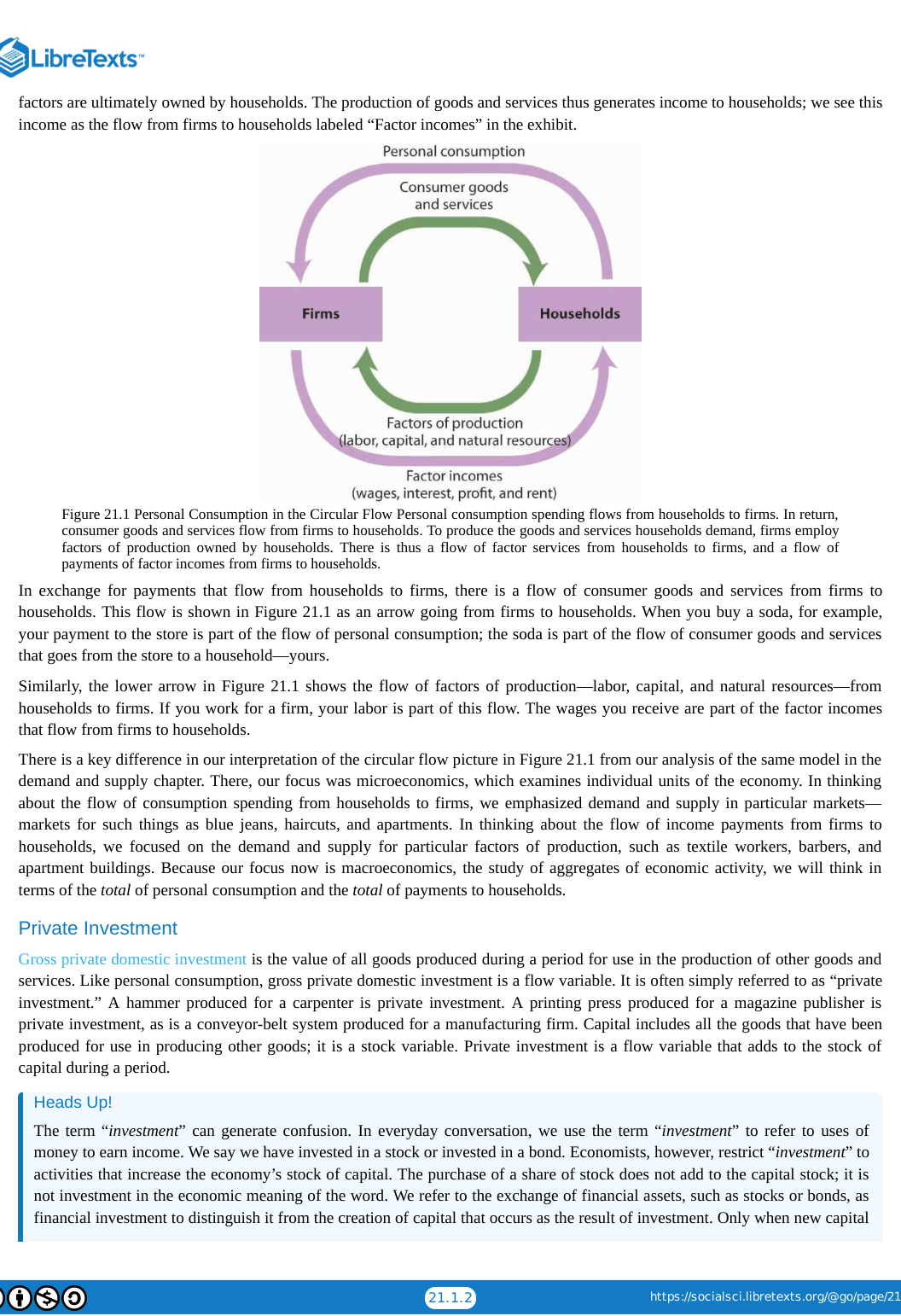
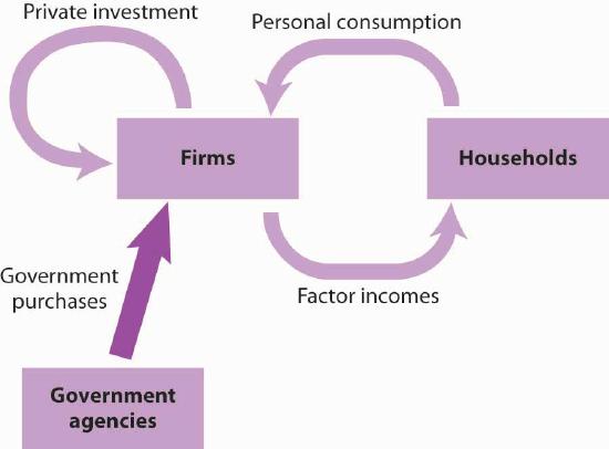
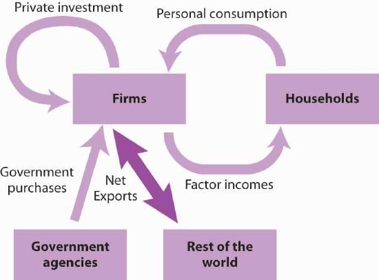
- The circular flow model illustrates the continuous interaction and adjustment between households and firms within an economy.
- Economic activity is defined as a process of exchange where firms provide goods and services while households provide factors of production like labor and capital.
- Product markets represent the top half of the cycle where households demand goods, while factor markets represent the bottom half where firms demand resources.
- The model demonstrates how markets are interrelated, showing that a change in demand for a consumer product directly impacts the demand for the labor required to produce it.
- While simplified by omitting government and foreign sectors, the model accurately reflects the millions of individual exchanges that constitute a private domestic economy.
The circular flow model shows that goods and services that households demand are supplied by firms in product markets.
Market Equilibrium and Obesity Trends
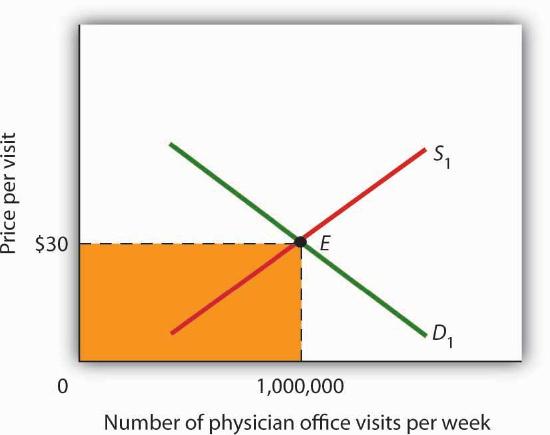
- Equilibrium price is established at the intersection of supply and demand curves where quantity supplied equals quantity demanded.
- Market imbalances such as surpluses and shortages exert downward or upward pressure on prices to restore equilibrium.
- Shifts in demand or supply curves independently predict changes in price and quantity, but simultaneous shifts require knowing the magnitude of each change.
- The circular flow model illustrates the interconnectedness of product and factor markets within an economy.
- Economic principles of supply and demand are being applied to analyze the rising rates of obesity in the United States.
- Research suggests obesity now has a stronger correlation with chronic medical conditions and healthcare costs than smoking or alcoholism.
Obesity appears to have a stronger association with the occurrence of chronic medical conditions, reduced physical health-related quality of life and increased health care and medication expenditures than smoking or problem drinking.
Economics of Rising Obesity
- Increased demand for food is driven by sedentary lifestyles and higher income levels, contributing to roughly 60% of weight gain.
- Modern life requires fewer calories to prepare food or earn the income to purchase it, compounding the physiological impact of caloric intake.
- Despite rising demand, the relative price of food has actually declined by 0.2% annually since World War II.
- Agricultural innovation has caused a massive rightward shift in the supply curve, which outweighs the shift in demand and lowers equilibrium prices.
- The remaining 40% of weight gain is attributed to these technological advancements in food production that make calories cheaper and more accessible.
What more apt picture of our sedentary life style is there than spending the afternoon watching a ballgame on TV, while eating chips and salsa, followed by a dinner of a lavishly topped, take-out pizza?
Market Equilibrium and Dynamics
- The law of demand dictates that price increases reduce quantity demanded, while the law of supply suggests price increases generally boost quantity supplied.
- Market equilibrium is reached at the intersection of demand and supply curves, where the quantity demanded exactly matches the quantity supplied.
- Prices above equilibrium create surpluses, while prices below equilibrium result in shortages, both of which are typically temporary in a functioning market.
- Changes in the underlying determinants of demand and supply shift the curves, resulting in new equilibrium prices and output levels.
- Economic logic can be applied to real-world safety issues, such as how airfare pricing indirectly influences highway fatality rates through substitution effects.
Usually, market surpluses and shortages are short-lived.
Economic Principles in Practice
- The text presents real-world scenarios to test the application of supply and demand models, such as how low-carb diet trends impact egg prices.
- It contrasts public perception of price gouging during peak travel seasons with the economic reality of seasonal demand shifts.
- Market dynamics are explored through historical shifts, including the rise of Vietnam as a coffee exporter and the transition of skim milk from hog feed to a primary consumer product.
- The relationship between substitute and complementary goods is examined through the correlation between rising cigarette prices and increased food consumption.
- Labor market imbalances are analyzed using the example of Indian outsourcing, where demand for college graduates outpaces the available supply.
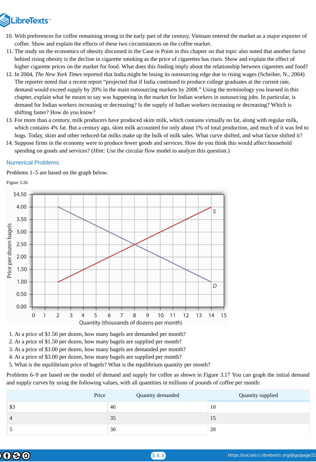
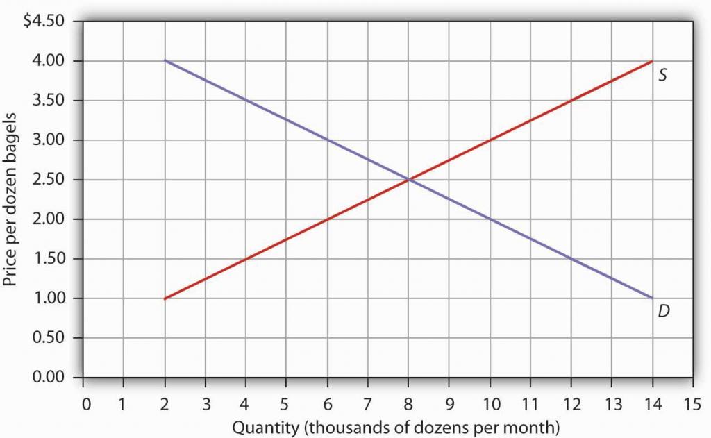
- Numerical problems provide a framework for calculating equilibrium price and quantity using specific data points for commodities like bagels and coffee.
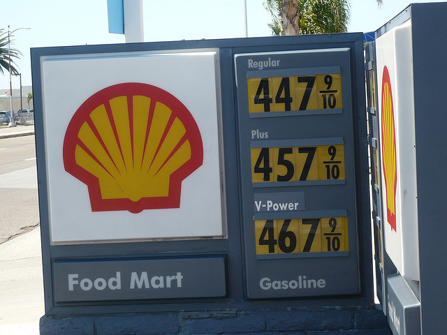
I think the gas companies just use any excuse to jack up prices, and they’re doing it again now.
Market Equilibrium and Applications
- The text provides practical exercises for calculating shifts in demand and supply curves based on specific price and quantity changes.
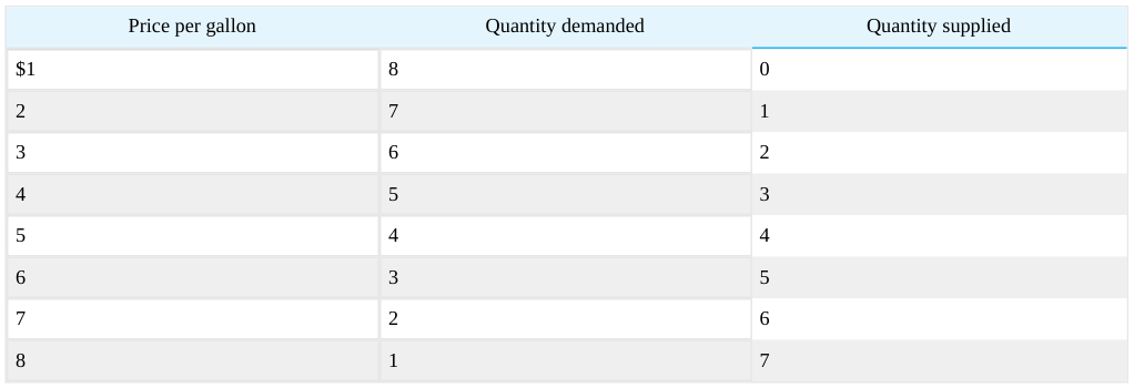
- Students are tasked with identifying market surpluses and shortages by comparing quantity demanded and quantity supplied at various price points.
- A gasoline market case study illustrates how equilibrium is reached when quantity demanded equals quantity supplied at a specific price.
- The material introduces the concept of simultaneous shifts in both demand and supply, challenging students to predict outcomes for price and quantity.
- The chapter transitions into real-world applications, including government interventions like price floors and ceilings and the health-care market.
- A focus is placed on how external factors, such as technological change, can be modeled using standard demand and supply frameworks.
If the demand curve shifts as in problem 13 and the supply curve shifts as in problem 14, without drawing a graph or consulting the data, can you predict whether equilibrium price increases or decreases?
Evolution of the PC Market
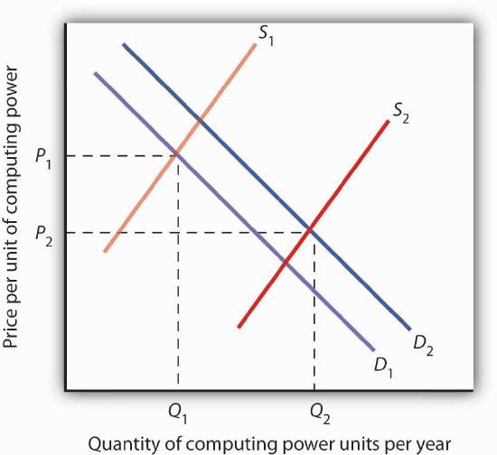
- The model of demand and supply is used to analyze rapid price and quantity shifts in markets like crude oil, stocks, and personal computers.
- Technological advancement in the computer industry has been so rapid that economists must use 'quality-adjusted' metrics to compare hardware across different eras.
- The 'halving time' for the price of quality-adjusted desktop computers accelerated from 50 months in the late 70s to just 24 months by the late 90s.
- Explosive growth in hardware capability is evidenced by CPU speeds and hard drive capacities increasing by thousands of percentage points within single decades.
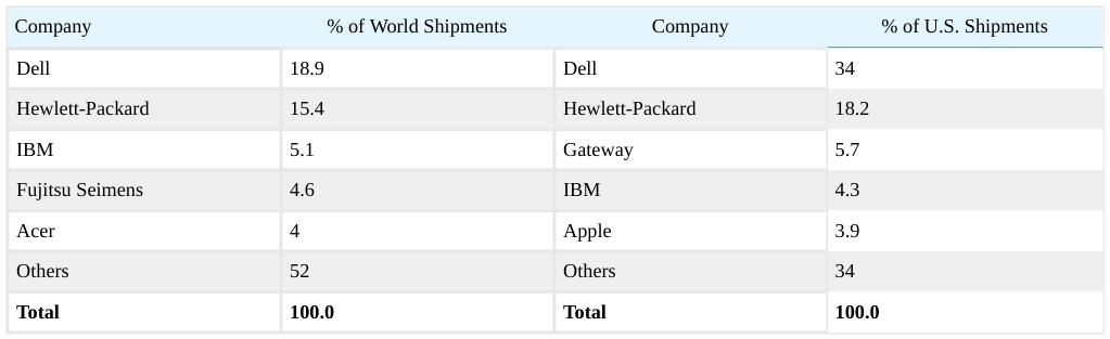
- The industry transitioned from a near-monopoly held by IBM in the mainframe era to a highly competitive global market with numerous manufacturers.
In 1984, just 8.2% of U.S. households owned a personal computer. By 2007, Google estimates that 78% did.
Market Shifts in Tech and Oil
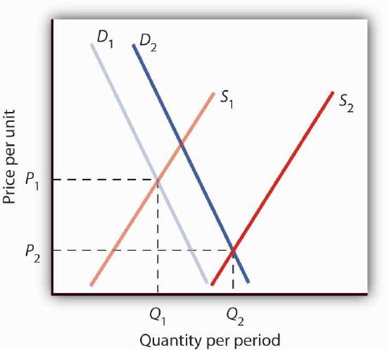
- The personal computer market experienced a massive rightward supply shift due to technological advancements and increased competition, lowering prices despite rising demand.
- Computer demand grew simultaneously as rising incomes and new technologies like VoIP and RFID expanded the utility of computing power.
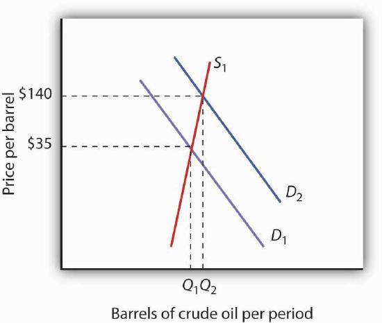
- Crude oil prices spiked to $147 per barrel in 2008, driven primarily by surging global demand from emerging economies like China outpacing production capacity.
- Rising energy costs act as a universal supply-side shock, shifting supply curves for nearly all goods and services to the left and increasing general price levels.
- The volatility of the oil market was demonstrated when the 2008 economic slowdown caused a rapid demand reversal, dropping prices from record highs to below $60 in months.
Higher oil prices also increase the cost of producing virtually every good or service, as at a minimum, the production of most goods requires transportation.
The Circular Flow of Capital
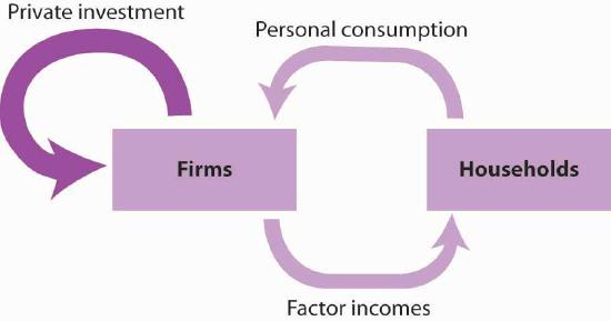
- The circular flow model posits that households supply factors of production, including capital, to firms.
- In exchange for providing capital, firms pay income back to the households.
- In practical reality, many large corporations like General Motors and Wal-Mart directly own their physical capital.
- There is a conceptual tension between the theoretical model of household ownership and the reality of corporate ownership.
- The relationship between firms and households remains the foundational link in macroeconomic resource distribution.
General Motors owns its assembly plants, and Wal-Mart owns its stores; these firms therefore own their capital.
Mechanics of the Stock Market
- Households ultimately own all capital through their ownership of firms, whether as sole proprietorships, partnerships, or corporations.
- While most U.S. firms are small businesses, corporations produce approximately 90% of the nation's total output and own the majority of capital.
- Corporations only receive direct funding during an Initial Public Offering (IPO); subsequent trading occurs on the secondary market without further funding to the firm.
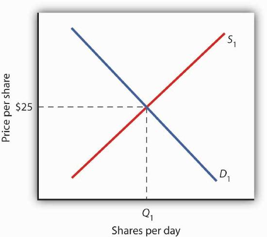
- Stock prices are determined by the interaction of supply and demand, where the supply curve represents the willingness of current owners to sell at various price points.
- The stock market functions as a global network of institutions where brokers and traders match buy and sell orders to reach equilibrium prices.
The process through which shares of stock are bought and sold can seem chaotic.
Mechanics of Stock Valuation
- Stock prices are determined by the intersection of supply and demand curves, representing the equilibrium between buyers and sellers.
- A share of stock represents a claim on a company's future profits, which are either reinvested as retained earnings or distributed as dividends.
- Because future profits are uncertain, stock prices are essentially market estimates based on product demand, production costs, and management quality.
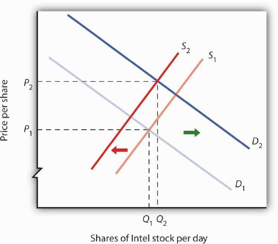
- Shifts in supply and demand are primarily driven by changes in expectations; positive news shifts demand right and supply left, raising the price.
- Broader macroeconomic factors, such as demographic shifts toward retirement and overall economic health, influence general market price levels.
At the equilibrium price, the number of shares supplied by people who think holding the stock no longer makes sense just balances the number of shares demanded by people who think it does.
Market Volatility and Information
- Stock prices are constantly adjusted based on a continuous stream of new information, ranging from corporate profit reports to global geopolitical events.
- Technological advancements and shifts in global demand, such as the 2008 oil price fluctuations, demonstrate how supply and demand curves dictate equilibrium prices.
- Higher energy costs, like rising gasoline prices, create a systemic impact by shifting supply curves leftward, increasing prices while reducing output across industries.
- The equilibrium price of a stock represents a balance between market participants with opposing views on the asset's intrinsic value.
- Major disasters and 'complete surprises' like the 9/11 attacks cause dramatic short-term market declines by sapping consumer confidence and introducing extreme uncertainty.
The attacks on 9/11 provoked fear and uncertainty—two things that are certain to bring stock prices down, at least until other events and more information cause expectations to change again in this very responsive market.
Market Equilibrium and Price Controls
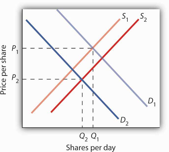
- Negative information regarding a corporation's profitability causes a simultaneous increase in stock supply and a decrease in demand.
- While market shifts clearly drive down equilibrium prices, the final impact on equilibrium quantity depends on the relative magnitude of the shifts.
- Markets naturally tend toward equilibrium, where prices adjust to eliminate temporary surpluses and shortages.
- Governments often intervene in markets to artificially maintain prices above or below the natural equilibrium due to public pressure.
- Price floors in agriculture and price ceilings in rental markets serve as primary examples of government intervention and its consequences.
Surpluses and shortages of goods are short-lived as prices adjust to equate quantity demanded with quantity supplied.
Agricultural Price Floors
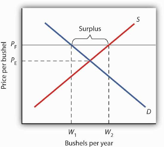
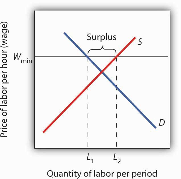
- A price floor is a government-mandated minimum price set above the market equilibrium to prevent prices from falling.
- Setting a price floor above equilibrium results in a persistent surplus because the quantity supplied exceeds the quantity demanded.
- If a price floor is set below the equilibrium price, it remains irrelevant as it does not prevent the market from reaching its natural balance.
- Technological advancements in farming have significantly increased global production capacity, leading to downward pressure on crop prices.
- Farmers have successfully lobbied for these price floors to protect their income from the price-reducing effects of increased efficiency.
While such price reductions have been celebrated in computer markets, farmers have successfully lobbied for government programs aimed at keeping their prices from falling.
Agricultural Economics and Policy
- Technological advances have shifted the agricultural supply curve rightward far more significantly than the modest demand increases driven by population and income growth.
- The disparity between high supply and low demand growth has led to a long-term historical trend of falling equilibrium prices for agricultural goods.
- Farmers face extreme income instability due to short-term volatility caused by weather events and sudden shifts in international trade policy.
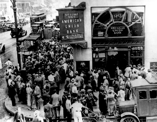
- The Great Depression served as a catalyst for federal intervention, as plummeting prices left over half of all farm loans in default by 1932.
- Government interventions have evolved from direct surplus purchasing and storage to 'target price' systems that pay farmers the difference between market rates and guaranteed minimums.
- To manage the surpluses created by price floors, the government often mandates acreage restrictions and conservation compliance from participating farmers.
Prices received by farmers plunged nearly two-thirds from 1930 to 1933.
Agricultural Subsidies and Reform
- Agricultural price support programs result in higher costs for consumers and significant government expenditure.
- U.S. federal spending on agriculture averaged over $22 billion annually between 2003 and 2007, costing roughly $70 per person.
- Farm aid often benefits large-scale producers rather than small farmers because subsidies are typically based on production volume.
- The 1996 FAIR Act attempted to phase out price supports to encourage market-based farming, but falling prices led to emergency aid.
- The 2008 farm bill increased subsidies to $40 billion while introducing the first income-based eligibility limits for wealthy farmers.
However, since farm aid has generally been allotted on the basis of how much farms produce rather than on a per-farm basis, most federal farm support has gone to the largest farms.
The Mechanics of Rent Control
- Rent control functions as a price ceiling designed to keep housing costs below market equilibrium for tenants.
- While primarily a local phenomenon in the U.S., rent control is pervasive across Europe and many developing nations.
- Economic models demonstrate that setting a price ceiling below equilibrium inevitably creates a persistent shortage of available units.
- Lower rents increase the quantity of housing demanded by encouraging individuals to live alone rather than with parents or roommates.
- On the supply side, artificially low rents discourage property owners from maintaining units or offering them to the rental market.
- The flexibility of these laws varies, with some cities allowing increases for improvements while others exempt newer constructions.
Even though an aerial photograph of a city would show apartments to be fixed at a point in time, owners of those properties will decide how many to rent depending on the amount of rent they anticipate.
Consequences of Rent Control
- Rent control creates a persistent shortage of apartments because the quantity demanded at the price ceiling exceeds the quantity supplied.
- The shortage leads to 'backdoor' payments such as exorbitant security deposits, forced furniture purchases, or illegal 'key' payments.
- Current occupants are disincentivized from moving, which reduces tenant mobility and creates a gap between controlled and uncontrolled units.
- The policy often fails its target demographic by benefiting long-term residents regardless of income rather than the poor.
- Administrative and enforcement costs add a significant burden to the government managing these price distortions.
- Direct income subsidies are suggested as a more efficient alternative to help low-income tenants without disrupting market mechanisms.
The monthly rent is $500 and the key price is $3,000.
Price Controls and Ethanol Policy
- Price floors set above equilibrium create persistent surpluses, often requiring governments to purchase excess goods or restrict production.
- Price ceilings set below equilibrium result in shortages and can lead to 'backdoor' arrangements like bribes or forced rentals.
- The U.S. government has heavily subsidized corn production since 1938, transitioning from food support to massive ethanol fuel mandates.
- Critics argue that corn-based ethanol is energy-inefficient, requiring nearly as much energy to produce as it eventually provides.
- The diversion of crops from food to fuel contributes to global environmental degradation and rising food prices that impact the world's poor.
Filling the 25-gallon tank of an SUV with pure ethanol requires over 450 pounds of corn—which contains enough calories to feed one person for a year.
Market Interventions and Health Costs
- Corn-based ethanol production is criticized for its inefficiency and impact on global food prices, yet it remains heavily supported by government subsidies.
- Minimum wage laws set above equilibrium create a labor surplus while inadvertently increasing demand and wages for skilled workers who serve as substitutes.
- U.S. health-care spending has seen a massive structural shift, rising from 5% of total output in 1960 to over 15% by the early 2000s.
- The presence of third-party payers significantly alters the traditional supply and demand dynamics within the health-care market.
- Economic models of price floors and ceilings help explain why certain sectors, like agriculture and labor, experience persistent surpluses or shortages.
Nonetheless, it is clear that corn-based ethanol is no free lunch.
Economics of Third-Party Payers
- The health-care industry is a vast network of markets for diverse goods and services, ranging from complex surgeries to simple aspirin.
- In a standard market model, the equilibrium price and quantity for physician visits are determined by the intersection of supply and demand.
- Health insurance introduces a third-party payer system that significantly lowers the out-of-pocket cost for the consumer.
- Lowering the consumer's cost from the equilibrium price to a fixed co-pay increases the quantity of services demanded.
- To meet this increased demand, insurers must pay a premium to providers, resulting in a higher total price per visit than the original equilibrium.
- The presence of third-party payers leads to a substantial increase in total weekly spending within the health-care market.
When you get a cold, do you go to the doctor? Probably not, if it is a minor cold. But if you feel like you are dying, or wish you were, you probably head for the doctor.
Impact of Third-Party Payers
- Insurance and third-party payers decouple the price paid by consumers from the price received by suppliers.
- Lower out-of-pocket costs for consumers lead to a significant increase in the quantity of services demanded.
- Suppliers require higher total payments to meet increased demand, resulting in a rise in total market spending.
- This economic model applies beyond healthcare to other sectors like higher education through scholarships and subsidies.
- The expansion of healthcare spending represents a rising opportunity cost, diverting resources from other goods and services.
In markets with third-party payers, an equilibrium is achieved, but it is not at the intersection of the demand and supply curves.
The Oregon Health Plan
- The health-care industry faces a fundamental dilemma between providing universal insurance and controlling the resulting surge in spending.
- Oregon attempted to manage Medicaid costs by prioritizing medical treatments and refusing to fund those deemed less essential or cost-effective.
- The state created a ranked list of over 700 condition-treatment pairs, setting a 'line in the sand' for what the government would cover.
- Early implementation led to ethical controversy when the state refused to fund a life-saving bone marrow transplant for a child in favor of prenatal care.
- Research showed that the rationing system was largely bypassed in practice as physicians found ways to treat excluded conditions alongside covered ones.
- Ultimately, the plan expanded coverage without significant rationing because the state government increased revenues to fund the rising costs.
The decision turned out to be a painful one; the first year, a seven-year-old boy with leukemia, who might have been saved with a bone marrow transplant, died.
Oregon's Health Care Lottery
- Explicitly listing excluded medical treatments created political pressure that inadvertently drove up program costs.
- Severe budgetary constraints forced Oregon to shift from rationing services to drastically reducing the number of insured individuals.
- The number of people covered by the state plan plummeted from over 100,000 to approximately 17,000 due to funding cuts.
- Oregon's uninsured rate rose significantly from 11% in 1996 to 16% by 2008 as a direct result of these policy shifts.
- In 2008, the state implemented a lottery system to allocate a few thousand new openings among 130,000 eligible applicants.
- Economic models show that third-party payers increase total spending by decoupling the price paid by consumers from the cost required by providers.
More than 90,000 people queued up, hoping to be lucky winners.
Market Dynamics and Price Controls
- Technological advancements and new market entrants have shifted the supply curve for personal computers, making them affordable household staples.
- Global demand fluctuations, particularly from emerging economies like China, drive significant volatility in crude oil and gasoline prices.
- Stock prices function as real-time market estimates of a firm's future profitability, reacting instantly to new information.
- Government-imposed price floors and ceilings often result in unintended consequences like persistent surpluses or chronic shortages.
- The presence of third-party payers in the health care market artificially inflates both the quantity of services consumed and total national spending.
We saw that interfering with the market mechanism may solve one problem but often creates other problems at the same time.
Economic Policy and Market Dynamics
- The text explores how historical wage freezes led to the rise of employer-financed retirement plans as non-taxable benefits.
- It examines the impact of political stability on the elasticity of the global oil supply curve and its subsequent effects on consumers.
- The relationship between technological advancement and government price supports is analyzed, specifically within the dairy and agricultural sectors.
- Market interventions such as rent controls, price ceilings on oil, and healthcare subsidies are evaluated for their unintended consequences on low-income populations.
- The text provides numerical problems to illustrate how price floors and ceilings create surpluses or shortages in commodities like corn.
The Internal Revenue Service went along with this and ruled that employer-financed retirement plans were not taxable income.
Market Controls and Elasticity
- The text provides practice problems for analyzing the effects of price floors on agricultural surpluses and government spending.
- A hypothetical apartment market dataset is used to illustrate equilibrium and the consequences of rent ceilings.
- Rent ceilings are shown to create discrepancies between the number of apartments demanded and the actual supply available.
- The concept of price elasticity of demand is introduced to quantify how much quantity demanded changes in response to price shifts.
- Elasticity is defined as the percentage change in quantity demanded divided by the percentage change in price, assuming all other factors remain constant.
- The curriculum outlines various degrees of responsiveness, ranging from perfectly inelastic to perfectly elastic demand.
We know from the law of demand how the quantity demanded will respond to a price change: it will change in the opposite direction. But how much will it change?
Price Elasticity of Demand
- Price elasticity of demand measures the responsiveness of quantity demanded to price changes along a demand curve.
- Because price and quantity move in opposite directions, the price elasticity of demand is mathematically always a negative value.
- Economists often use absolute values for elasticity, though this text retains the minus sign to maintain mathematical consistency.
- A critical distinction exists between slope and elasticity: slope measures absolute change, while elasticity measures percentage change.
- On a linear demand curve, the slope remains constant while the price elasticity of demand varies at different points.
- Calculating elasticity requires determining the percentage changes in price and quantity between two specific points on a curve.
Be careful not to confuse elasticity with slope.
Calculating Arc Elasticity
- The demand curve illustrates the inverse relationship between price changes and the quantity of goods or services demanded.
- Arc elasticity measures responsiveness by using the average value of variables between two points as the denominator.
- This method ensures that the elasticity value remains consistent regardless of the direction of the change between two points.
- Percentage changes in quantity and price are calculated relative to their respective midpoints to avoid mathematical bias.
- The provided example demonstrates a price elasticity of demand of -3.00 for a specific shift in transit ride pricing.
The arc elasticity method has the advantage that it yields the same elasticity whether we go from point A to point B or from point B to point A.
Arc Elasticity and Linear Demand
- The arc elasticity method estimates elasticity at the midpoint between two points on a demand curve.
- To maintain accuracy, arc elasticity should only be applied to small changes in independent variables.
- Standard percentage change calculations yield different results depending on the direction of the change.
- The arc elasticity formula uses average price and quantity to ensure the result is consistent regardless of direction.
- On a linear demand curve, the price elasticity of demand decreases in absolute value as one moves downward and to the right.
By using the average quantity and average price to calculate percentage changes, the arc elasticity approach avoids the necessity to specify the direction of the change.
Elasticity Along Linear Demand
- Price elasticity of demand is not constant but varies at different points along a linear demand curve.
- At higher prices and lower quantities, the absolute value of price elasticity is relatively large.
- As price decreases and quantity increases, the absolute value of the elasticity measure consistently declines.
- Equal changes in price and quantity result in different percentage changes depending on the starting position on the curve.
- The midpoint of a linear demand curve typically represents unit elasticity, where the value equals -1.00.
- Moving down and to the right along the curve shifts the demand from elastic to inelastic territory.
As we move down the demand curve, equal changes in quantity represent smaller and smaller percentage changes, whereas equal changes in price represent larger and larger percentage changes, and the absolute value of the elasticity measure declines.
Price Changes and Total Revenue
- Total revenue is calculated as the price per unit multiplied by the quantity sold, making it sensitive to shifts in consumer demand.
- A change in price triggers two opposing forces: the price effect and the quantity effect, which move in opposite directions.
- The impact of a price hike on revenue is inconsistent; it can cause total revenue to rise, fall, or remain entirely unchanged.
- Specific examples like gasoline show that higher prices can increase revenue if the drop in consumption is minimal.
- In contrast, products like diet cola demonstrate that a price increase can lead to a net loss in revenue if consumers are highly sensitive to cost.
- The ultimate predictor of whether a price change will benefit a seller is the price elasticity of demand.
Even though people consume less gasoline at $4.25 than at $4.00, total revenue rises because the higher price more than makes up for the drop in consumption.
Elasticity and Total Revenue
- Economists categorize price elasticity into three types based on absolute value: elastic (greater than 1), unit elastic (equal to 1), and inelastic (less than 1).
- Total revenue movement depends on whether the percentage change in price or quantity is larger.
- When demand is price elastic, total revenue moves in the direction of the quantity change because quantity is more sensitive to price shifts.
- Inelastic demand, such as that for gasoline, results in total revenue moving in the same direction as the price change.
- Unit price elasticity represents a perfect balance where price and quantity changes offset each other, leaving total revenue unchanged.
- The arc elasticity method provides a mathematical framework to calculate these relationships using average price and quantity.
Total revenue will move in the direction of the variable that changes by the larger percentage.
Elasticity and Total Revenue
- Unit price elasticity occurs when the percentage change in quantity demanded exactly offsets the percentage change in price, leaving total revenue unchanged.
- In the case of diet cola, a price increase led to a larger percentage drop in quantity, demonstrating elastic demand where total revenue follows the direction of quantity change.
- A linear demand curve is divided into two distinct regions: the upper half is price elastic, while the lower half is price inelastic.
- Total revenue can be visualized as the area of a rectangle formed by price and quantity; this area increases during price cuts in the elastic region but decreases in the inelastic region.
- At the exact midpoint of any linear demand curve, the demand is unit price elastic, representing the transition point for revenue trends.
Notice that the area gained in moving to the rectangle at B is greater than the area lost; total revenue rises to $42,000.
Constant Price Elasticity Curves
- Perfectly inelastic demand is represented by a vertical curve where price changes have zero effect on the quantity demanded.
- Insulin serves as a real-world approximation of perfectly inelastic demand because patients require a specific amount regardless of price fluctuations.
- Perfectly elastic demand is represented by a horizontal curve where even minute price changes cause quantity demanded to drop to zero.
- Standardized commodities like wheat exemplify perfectly elastic demand because individual producers must accept the prevailing market price.
- Nonlinear demand curves can maintain a constant negative elasticity value across their entire range, unlike standard linear curves.
- The primary determinants of price elasticity include the availability of substitutes, budget importance, and the passage of time.
A diabetic will not consume more insulin as its price falls but, over some price range, will consume the amount needed to control the disease.
Determinants of Price Elasticity
- The availability of close substitutes significantly increases price elasticity by allowing consumers to easily switch brands when prices rise.
- Broad categories of goods, like gasoline, tend to be price inelastic because they lack direct substitutes, whereas specific brands within those categories are highly elastic.
- The proportion of a household budget spent on an item dictates its elasticity; expensive items like jeans see larger demand shifts than inexpensive items like pencils.
- Time is a critical factor in consumer response, as long-run price elasticity is almost always greater than short-run elasticity due to the ability to adjust habits or technology.
- OPEC leverages the short-term inelasticity of crude oil by restricting supply to drive up prices and maximize total revenue for member nations.
A change in pencil prices, in contrast, might lead to very little reduction in quantity demanded simply because pencils are not likely to loom large in household budgets.
Price Elasticity and Time
- Global data on crude oil demand demonstrates that price elasticity is consistently higher in the long run than in the short run across various nations.
- The price elasticity of demand measures how quantity demanded responds to price changes, categorized as inelastic, unit elastic, or elastic based on absolute values.
- Total revenue movements depend on elasticity: revenue increases with price hikes if demand is inelastic, but decreases if demand is elastic.
- Factors influencing elasticity include the availability of substitutes, the budget share of the good, and the duration of the adjustment period for consumers.
- A practical application in public transit shows that a fare increase may raise revenue in the short term (inelastic demand) but decrease it in the long term (elastic demand).
Your only hope is to increase revenue. Would a fare increase boost revenue?
Elasticity of Red Light Violations
- Economists studied the impact of increased traffic fines on driver behavior in Israel and San Francisco to determine the price elasticity of running red lights.
- The implementation of intersection cameras ensured a high probability of citation, making the 'price' of the violation more certain for drivers.
- In Israel, a 150 percent increase in fines resulted in a 31.5 percent reduction in violations, yielding an elasticity of -0.21.
- Demographic analysis revealed that younger drivers and lower-income individuals were more responsive to fine increases than older or wealthier drivers.
- The study concludes that drivers act rationally; as the cost of a dangerous behavior increases, the frequency of that behavior decreases.
- The combination of higher fines and automated enforcement via cameras serves as an effective tool for reducing traffic fatalities.
We can think of driving through red lights as an activity for which there is a demand—after all, ignoring a red light speeds up one’s trip.
Elasticity and Consumer Responsiveness
- Price elasticity of demand increases over time as consumers find more alternatives, such as carpooling or moving in response to transit fare hikes.
- Short-term demand for commuter rail is inelastic, meaning a price increase leads to a relatively small drop in ridership and an increase in total revenue.
- Long-term demand becomes elastic, resulting in a significant ridership decline that eventually causes total revenue to fall.
- Total revenue and total spending are functionally identical measures, differing only in whether the focus is on the seller's income or the buyer's costs.
- Income elasticity of demand measures how quantity demanded shifts in response to changes in consumer income, distinguishing between normal and inferior goods.
- Cross price elasticity of demand evaluates how the price change of one good affects the demand for related substitutes or complements.
Total revenue falls after a few years, since demand changes and becomes price elastic.
Income and Cross Price Elasticity
- Income elasticity of demand measures how quantity demanded shifts at a specific price in response to changes in consumer income.
- Normal goods have positive income elasticity, meaning demand increases as income rises, common in sectors like housing and medical services.
- Inferior goods, such as beans or public transit, exhibit negative income elasticity where higher income leads to decreased demand.
- Cross price elasticity of demand quantifies how the price change of one good affects the demand for a different, related good.
- Positive cross price elasticity identifies substitute goods, while negative cross price elasticity identifies complementary goods.
- Unlike price elasticity which tracks movement along a curve, both income and cross price elasticities represent shifts of the demand curve itself.
A reduction in the price of salsa, for example, would increase the demand for chips, suggesting that salsa is a complement of chips.
Elasticity and Market Relationships
- Local television and radio advertising function as clear substitutes in the marketplace.
- A cross price elasticity of 1.0 indicates that television demand rises proportionally with radio price increases.
- Income elasticity determines whether a good is classified as normal or inferior based on positive or negative values.
- Cross price elasticity identifies whether two goods are substitutes or complements.
- The terms 'elastic' and 'inelastic' are strictly reserved for price elasticity of demand rather than income or cross price measures.
A 10 per cent increase in the price of local radio advertising led to a 10 per cent increase in demand for local television advertising.
Elasticity and Tobacco Policy
- Income elasticity measures demand responsiveness to income changes, distinguishing between normal and inferior goods.
- Cross price elasticity identifies the relationship between goods, defining them as substitutes, complements, or unrelated.
- Teenagers exhibit a significantly higher price elasticity of demand for cigarettes than adults because tobacco costs consume a larger portion of their income.
- The 1998 Master Settlement Agreement led to a 48 percent increase in cigarette prices, resulting in a sharp decline in teenage smoking rates.
- Health economists prioritize price-based interventions for youth because most smokers begin as teenagers and underestimate the long-term difficulty of quitting.
Teens tend to underestimate the danger of smoking and to overestimate their likely ability to quit smoking when they choose to do so.
Elasticity and Teen Smoking
- State excise taxes on cigarettes vary dramatically across the United States, ranging from 2.5 cents to over 1.50 dollars per pack.
- Teenagers exhibit a high level of price responsiveness, making excise tax hikes a potentially effective tool for reducing youth smoking rates.
- A significant unintended consequence of raising cigarette prices is the potential for teens to switch to smokeless tobacco products.
- Research indicates a high cross price elasticity of 1.2 for young males, meaning a 10% rise in cigarette prices causes a 12% rise in smokeless tobacco use.
- The text also introduces the concept of price elasticity of supply, highlighting how time and market conditions affect producer responsiveness.
It is estimated that for young males the cross price elasticity of smokeless tobacco with respect to the price of cigarettes is 1.2—a 10% increase in cigarette prices leads to a 12% increase in young males using smokeless tobacco.
Price Elasticity of Supply
- Price elasticity of supply measures how responsive the quantity supplied of a good is to changes in its price.
- When demand increases, a more responsive supply curve results in a smaller price increase and a larger quantity increase compared to an inelastic supply curve.
- The price elasticity of supply is typically positive because price and quantity supplied generally move in the same direction.
- Supply is categorized as elastic if the value is greater than 1, unit elastic if equal to 1, and inelastic if less than 1.
- Extreme cases include perfectly inelastic supply, where quantity is fixed regardless of price, and perfectly elastic supply, where quantity is infinite at a specific price.
The supply of Beatles’ songs is perfectly inelastic because the band no longer exists.
Time and Supply Elasticity
- The price elasticity of supply is heavily dependent on the time horizon available for producers to respond to price changes.
- In the short run, supply is often inelastic because immediate capacity is limited to minor adjustments like reducing vacancy rates or quick renovations.
- Long-term supply is significantly more elastic as it allows for major capital investments, such as building new apartment complexes or converting existing structures.
- Labor supply presents a unique case where elasticity can be negative, meaning higher wages may actually lead to a decrease in hours worked.
- The 'backward-bending' labor supply occurs when high-income earners prioritize leisure time over the marginal utility of additional income.
- Elasticity measures across various goods—from crude oil to illicit drugs—demonstrate how differently markets react to price, income, and cross-product changes.
What makes this case interesting is that it has sometimes been found that the measured elasticity is negative, that is, that an increase in the wage rate is associated with a reduction in the quantity of labor supplied.
Price Elasticity of Supply
- The price elasticity of supply measures how the quantity of a good or service supplied responds to changes in its market price.
- Supply elasticity is generally positive and tends to increase over longer time horizons as producers gain more flexibility to adjust production.
- Labor supply elasticity varies significantly by profession, with lower-paying roles like child-care workers showing much higher elasticity than specialized medical roles.
- In certain high-paying professions, the labor supply curve can actually become negative if higher wages lead individuals to prioritize leisure over additional work.
- Empirical data shows a wide range of elasticities across goods, from highly inelastic crude oil and milk to highly elastic fresh tomatoes and lettuce.
In some very high-paying professions, the labor supply curve may have a negative slope, which leads to a negative price elasticity of supply.
Physician Labor Supply Elasticities
- Research indicates that the overall labor supply elasticity for young physicians is approximately 0.3, meaning a 10% wage increase results in only a 3% increase in hours worked.
- Female physicians exhibit a higher labor supply elasticity (0.5) compared to their male counterparts (0.2), likely due to lower average earnings in the sample.
- Younger physicians often maintain positive labor elasticities because high educational debt incentivizes working more as wages rise to facilitate loan repayment.
- In contrast to younger doctors, specialists show a negative elasticity of -0.3, suggesting they choose to work less as their income increases.
- Primary care physicians demonstrate an elasticity near zero, indicating their labor supply is largely unresponsive to changes in wage rates.
- Economic analysis of illicit substances suggests that marijuana, alcohol, and cocaine are normal goods, while heroin may be an inferior good.
Thus, for this sample of physicians, increases in wages have little or no effect on the amount the primary care doctors work, while a 10% increase in wages for specialists reduces their quantity of labor supplied by about 3%.
Economic Elasticity and Market Research
- The text provides an extensive bibliography of empirical studies focusing on price elasticity and demand across diverse industries.
- Research topics include the economic impacts of addictive substances such as tobacco, alcohol, and illicit drugs on public health.
- Several citations explore the intersection of public policy and consumer behavior, specifically regarding cigarette taxes and legal drinking ages.
- The list highlights econometric analyses of specific commodity markets, including meat, dairy, soft drinks, and Christmas trees.
- The section transitions into a summary of elasticity as a fundamental tool for measuring how dependent variables respond to changes in independent variables.
Elasticity is a measure of the degree to which a dependent variable responds to a change in an independent variable.
Fundamentals of Economic Elasticity
- Elasticity measures the percentage change in a dependent variable relative to a percentage change in an independent variable.
- Price elasticity of demand determines how total revenue shifts: it follows quantity in elastic markets and price in inelastic markets.
- Key determinants of demand elasticity include the availability of substitutes, budget importance, and the passage of time.
- Income and cross price elasticities use positive or negative signs to classify goods as normal, inferior, substitutes, or complements.
- Price elasticity of supply measures producer responsiveness, which is typically positive and increases over longer time horizons.
Total revenue moves in the direction of the quantity change if demand is price elastic, it moves in the direction of the price change if demand is price inelastic, and it does not change if demand is unit price elastic.
Elasticity Problems and Applications
- The text presents practical exercises for calculating price elasticity of supply and demand using real-world scenarios like child-care wages and cigarette taxes.
- Numerical problems explore the correlation between class attendance and academic performance, specifically calculating the elasticity of grades.
- Case studies on the orange juice market demonstrate how bumper crops and price cuts affect unit volume and total consumer spending.
- Restaurant management scenarios illustrate the relationship between price reductions, quantity demanded, and the resulting impact on total revenue.
- The exercises verify the economic principle that linear demand curves transition from elastic to inelastic as one moves from the upper to the lower half.
Economist David Romer found that in introductory economics classes a 10% increase in class attendance is associated with a 4% increase in course grade.
The Logic of Maximizing Behavior
- Economists assume that consumers and firms act as maximizers to achieve specific objectives like utility or profit.
- The concept of economic profit is defined as the difference between total revenue and opportunity costs.
- The marginal decision rule, involving marginal benefit and marginal cost, is the primary tool for understanding these choices.
- Maximization models are theoretical frameworks; economists do not claim people perform these complex calculations consciously.
- Human behavior is analyzed as being 'broadly consistent' with maximization models even if the actors are unaware of them.
- The transition from elasticity review to market efficiency highlights the shift from consumer response to behavioral logic.
People may not consciously seek to maximize anything, but they behave as though they do.
The Marginal Decision Rule
- Economic actors aim to maximize net benefit by subtracting opportunity costs from total benefits.
- Firms define net benefit as economic profit, which is total revenue minus total opportunity cost.
- The marginal decision rule dictates that an activity should increase if its marginal benefit exceeds its marginal cost.
- Net benefit is officially maximized at the specific point where marginal benefit equals marginal cost.
- All maximizing choices are subject to constraints, such as a consumer's budget or a firm's production capacity.
- This rule provides a universal framework for analyzing diverse choices, from buying fast food to manufacturing semiconductors.
The rule basically says this: If the additional benefit of one more unit exceeds the extra cost, do it; if not, do not.
The Economics of Study Time
- A student named Laurie Phan must allocate a fixed constraint of five hours between two different exams to maximize her total score gain.
- Total benefit is defined as the cumulative increase in exam points, which rises at a decreasing rate as more time is invested.
- Marginal benefit represents the specific point gain from each additional hour of study and is mathematically equivalent to the slope of the total benefit curve.
- The marginal benefit curve is downward-sloping, reflecting the principle that each subsequent hour of study yields fewer additional points than the hour before it.
- To accurately represent the transition between units of time, marginal values are plotted at the midpoints of the hourly intervals on a graph.
- This downward-sloping marginal benefit curve is a universal economic phenomenon applicable to the activities of both consumers and firms.
Notice that the total benefit curve rises, but by smaller and smaller amounts, as she studies more and more.
Marginal Benefits and Opportunity Costs
- The marginal benefit of an activity typically decreases as more time or resources are devoted to it, a concept known as diminishing returns.
- Economists assume individuals act as if they are calculating marginal costs and benefits, even if they do not use formal numerical scales.
- In a fixed-time scenario, the marginal cost of one activity is defined by the foregone marginal benefit of the alternative activity.
- Marginal cost curves generally slope upward because increasing one activity requires sacrificing increasingly productive time from another.
- The allocation of study time serves as a practical model for how individuals intuitively balance competing priorities to maximize total utility.
Economists do not assume that people have numerical scales in their heads with which to draw marginal benefit and marginal cost curves. They merely assume that people act as if they did.
The Marginal Decision Rule
- Reducing a secondary activity increases the forgone marginal benefits, effectively raising the marginal cost of the primary activity.
- The marginal decision rule is used to maximize the net benefit of any given activity.
- Optimal net benefit is achieved by increasing an activity until the marginal benefit equals the marginal cost.
- Graphically, the ideal allocation of time occurs at the intersection of the marginal benefit and marginal cost curves.
- In the provided example, the equilibrium is reached at three hours of economics study and two hours of accounting.
This rule says that, to maximize the net benefit of an activity, a decision maker should increase an activity up to the point at which marginal benefit equals marginal cost.
Marginal Benefit and Cost Curves
- Marginal benefit and marginal cost curves are used to calculate the total benefit, total cost, and net benefit of an activity.
- The total benefit of an action is represented by the sum of the areas of rectangles under the marginal benefit curve.
- Total cost is similarly derived by calculating the area under the marginal cost curve for a given quantity of time or effort.
- Equating marginal benefit to marginal cost is the primary mechanism for maximizing the net benefit of an activity.
- As the intervals of measurement become smaller, the sum of the rectangular areas more precisely matches the area under the continuous curves.
Suppose, instead of thinking in intervals of whole hours, we think in terms of smaller intervals, say, of 12 minutes.
Calculating Net Benefit and Deadweight Loss
- The area under a marginal benefit curve represents total benefit, while the area under a marginal cost curve represents total cost.
- As the intervals of measurement become smaller, the approximation of total benefit and cost via rectangles becomes increasingly precise.
- Maximum net benefit is achieved at the intersection of marginal benefit and marginal cost curves, represented by the area between the two curves.
- Deadweight loss occurs when an activity is performed at a level below the efficient equilibrium, resulting in forgone net benefits.
- Increasing an activity beyond the point where marginal benefit equals marginal cost creates a deadweight loss because costs exceed benefits for those additional units.
The loss in net benefits resulting from a failure to carry out an activity at the efficient level is called a deadweight loss.
The Marginal Decision Rule
- The marginal decision rule dictates that an activity should be increased if marginal benefit exceeds marginal cost and decreased if marginal cost exceeds marginal benefit.
- Net benefit is maximized at the specific point where marginal benefit exactly equals marginal cost, creating the largest possible gap between total benefit and total cost.
- A common misconception is that equating marginal benefit and cost results in zero net benefit, when it actually identifies the peak value of the objective.
- Total benefit and total cost can be visualized geometrically as the areas under their respective marginal curves.
- Economic decision-making assumes that individuals act rationally to maximize the value of a specific objective through incremental adjustments.
It is easy to make the mistake of assuming that if an activity is carried out up to the point where marginal benefit equals marginal cost, then net benefits must be zero.
Economics of Oil Spills
- Preventing oil spills involves a trade-off between environmental protection and the increased cost of consumer goods like gasoline.
- Economist Mark Cohen determined that the marginal benefit of preventing a gallon of spilled oil ($7.27) exceeded the marginal cost ($5.50), justifying stricter enforcement.
- Major disasters like the Exxon Valdez and the Prestige served as catalysts for significant legislative changes in the U.S. and the EU.
- The Oil Pollution Act of 1990 significantly increased shipper liability and mandated the use of double-hulled tankers.
- Regulatory tightening following major crises has successfully reduced the amount of oil spilled per barrel shipped by 30% over three decades.
The only way to prevent oil spills completely is to stop shipping oil. That is a cost few people would accept.
The Logic of Maximizing Behavior
- The marginal decision rule demonstrates that individuals maximize net benefit by adjusting behavior until marginal benefit equals marginal cost.
- Adam Smith's 'invisible hand' theory suggests that individual pursuit of self-interest can inadvertently promote the general interest of society.
- Economic efficiency is achieved when the net benefits of all economic activities, including both production and consumption, are maximized.
- A truly efficient allocation of resources requires competitive markets where no single buyer or seller controls the price.
- The existence of well-defined property rights is a fundamental condition for markets to achieve an efficient allocation of resources.
He said resources would be guided, as if by an “invisible hand,” to their best uses.
Property Rights and Market Efficiency
- Property rights establish the legal rules for how owners can use, manage, and control specific resources.
- A clear specification of ownership is the fundamental prerequisite for any market exchange to take place.
- The absence of enforceable property rights, such as the inability to prevent theft, would lead to the total collapse of retail markets.
- Exclusivity is a core requirement of property rights, allowing owners to prevent others from using a resource and providing an incentive for maintenance.
- Transferability is essential for economic efficiency as it allows owners to sell or lease resources to others through exchange.
- The combination of exclusive and transferable rights ensures that resources are allocated efficiently within a marketplace.
If it were the case for all grocery items, there would not be grocery stores at all.
Market Efficiency and Marginal Analysis
- A competitive market achieves efficiency when property rights are well-defined and transferable.
- The market demand curve serves as a representation of the marginal benefit to consumers based on their willingness to pay.
- The market supply curve represents the marginal cost to society, reflecting the value of goods foregone to produce the item.
- Profit-maximizing producers expand output until their marginal cost equals the market price.
- At equilibrium, marginal benefit equals marginal cost, resulting in the maximization of net benefit for society.
This marginal cost is considered in the economic sense—other goods and services worth $1.50 were not produced in order to make an additional pound of tomatoes available.
Consumer and Producer Surplus
- Market exchanges occur because both buyers and sellers expect to emerge from the transaction better off than before.
- Consumer surplus represents the difference between the total benefit consumers receive and the actual amount they pay for a good.
- Producer surplus is the difference between the total revenue received by sellers and the total cost of producing those goods.
- Net benefit to society is the sum of consumer and producer surplus, representing the total gain from economic activity.
- Social net benefit is maximized at the equilibrium point where the market demand and supply curves intersect.
Exchanges in the marketplace have a remarkable property: Both buyers and sellers expect to emerge from the transaction better off.
Efficiency Versus Equity
- Market responsiveness is directly tied to income levels, meaning the preferences of high-income individuals carry more weight in resource allocation.
- Efficiency and equity are distinct concepts; a market can be perfectly efficient even if 1% of the population controls and consumes all resources.
- Determining a fair distribution of income is a normative judgment based on personal values rather than a scientific or objective test.
- Most governments intervene in markets to redistribute income through taxes and welfare, suggesting a societal consensus that market-driven distribution is often unfair.
- An efficient allocation is always preferable to an inefficient one because it maximizes net benefits, which can theoretically be redistributed to benefit everyone.
For example, if 1% of the population controls virtually all the income, then the market will efficiently allocate virtually all its production to those same people.
Property Rights and Conservation
- The African elephant population faced a catastrophic decline in the late 20th century, dropping from 1.3 million to roughly 543,000 in just fifteen years.
- Traditional conservation methods, such as the CITES ivory ban and armed anti-poaching patrols, failed to stop the slaughter due to high black-market incentives.
- Nations like Botswana and Zimbabwe reversed this trend by establishing exclusive, transferable property rights through hunting licenses.
- Statistical analysis shows that elephant populations thrive in countries with stable political systems and clearly defined property rights.
- The white rhinoceros serves as another success story, with South African herds growing from 20 to over 7,000 through the sale of expensive hunting permits.
- The text concludes that establishing a market through property rights is a more effective preservation strategy than simple prohibition.
The tusks from a single animal could be sold for $2,000 in the black market—nearly double the annual per capita income in Kenya.
The Mechanics of Market Failure
- Market failure occurs when private decisions fail to achieve an efficient allocation of scarce resources, preventing the maximization of net benefits.
- Efficiency requires competitive markets and well-defined, transferable property rights so that decision makers face the true marginal costs and benefits.
- Noncompetitive markets allow individual buyers or sellers to influence prices, causing distortions where price no longer equals marginal cost.
- Public goods are defined by non-excludability and a marginal cost of zero for additional users, making them difficult for private markets to provide.
- Externalities, such as pollution from driving, represent costs not accounted for by the individual, leading to resource misallocation.
- The free rider problem arises with public goods because individuals can enjoy benefits without paying, necessitating government intervention.
A good for which the cost of exclusion is prohibitive and for which the marginal cost of an additional user is zero is a public good.
The Public Goods Dilemma
- Public goods are defined by non-excludability and zero marginal cost for additional users.
- A private firm providing national security would face the 'free rider' problem, where individuals consume the service without paying.
- Despite a total societal benefit of $4.5 billion exceeding a $1 billion cost, the market fails to signal the project's value.
- Efficient market pricing requires price to equal marginal cost, which for public goods is zero, making private profit impossible.
- The inherent nature of public goods prevents them from being effectively provided by private market mechanisms.
Recognizing the opportunity to consume the good without paying for it, most would be free riders.
Public Goods and Market Failure
- Private firms underproduce public goods because the free-rider problem prevents them from capturing the full value of the benefits provided.
- Government intervention can correct this inefficiency through direct provision, purchasing services from private firms, or offering subsidies.
- Taxation serves as the primary mechanism to finance public goods, effectively bypassing the issue of individuals refusing to pay voluntarily.
- The gap between the market-provided quantity and the efficient quantity of a public good results in a deadweight loss to society.
- A good's classification as 'public' or 'private' depends on its inherent characteristics, such as non-excludability, rather than which sector provides it.
- Subsidies for private charitable contributions are a common method for governments to encourage the production of public goods outside of direct agencies.
The fact that these goods are produced by a government agency does not make them a public good.
External Costs and Market Efficiency
- External costs occur when firms or individuals impose negative consequences on others outside of a formal market exchange.
- Media violence is cited as a significant external cost, with studies linking high exposure in children to increased real-world aggression and homicide rates.
- Market supply curves typically only reflect private marginal costs, ignoring the broader social impact of production activities like pollution.
- When external costs are not internalized, the market produces a higher quantity of goods at a lower price than is economically efficient.
- The gap between private costs and full social costs results in a deadweight loss, representing a failure of the market to allocate resources optimally.
- External benefits also exist, occurring when an action provides uncompensated advantages to others, such as the aesthetic value of a beautiful building.
By the time a child who spends the average amount of time watching television finishes elementary school, he or she will have seen 100,000 acts of violence, including 8,000 murders.
Managing External Costs
- Decision makers who generate external costs do not face the full financial burden of their actions, leading to inefficiently high levels of activity.
- When prices are artificially low because they exclude external costs, consumers tend to over-consume the resulting goods or services.
- Governments can intervene by imposing per-unit pollution fees to shift the supply curve and align production with the efficient quantity.
- Market-based solutions like purchasing pollution permits force firms to internalize the costs of their environmental impact.
- Direct regulation serves as an alternative to taxes, allowing authorities to order specific reductions in pollution or noise.
A person who turns his or her front yard into a garbage dump may be ordered to clean it up.
Common Property and Extinction
- Common property resources lack defined property rights, leading to a lack of individual incentives for preservation.
- The 19th-century survival of cattle versus the near-extinction of buffalo illustrates how ownership encourages herd maintenance and breeding.
- Individual buffalo hunters could not afford to conserve the population because any animal they spared would likely be killed by a competitor.
- The modern recovery of buffalo populations is attributed to the establishment of exclusive, transferable property rights and market demand.
- Species currently threatened with extinction, such as whales or elephants, are typically treated as common property resources.
- Preservation can be achieved either through government-imposed limits or by establishing private rights that delegate the task of conservation to owners.
Anyone who cut back on hunting in order to help to preserve the herd would lose income—and face the likelihood that other hunters would go on hunting at the same rate as before.
Externalities and Addictive Bads
- Public sector intervention can improve resource allocation efficiency by addressing free riders and external costs.
- Common property resources and activities with external benefits often fail to reach efficient levels in a pure market.
- While smokers impose external costs through healthcare and fires, they also provide external benefits by subsidizing retirement programs due to shorter lifespans.
- The concept of 'time inconsistency' suggests that smokers suffer from 'internalities,' where they seek immediate gratification but later regret the choice.
- If smoking is a rational choice, current excise taxes may already cover external costs; however, if it is irrational, much higher taxes could improve smoker welfare.
In an important way, however, smokers also generate external benefits. They contribute to retirement programs and to Social Security, then die sooner than nonsmokers.
Efficiency and Market Failure
- Economists assume individuals and firms make purposeful choices to maximize utility or profit using the marginal decision rule.
- Resource allocation is efficient when decision makers face all costs and benefits, maximizing the net benefit of every activity.
- Efficiency breaks down in the absence of competitive markets or when property rights are not exclusive and transferable.
- Market failures such as public goods, externalities, and common property resources often require public sector intervention.
- Deadweight loss represents the reduction in net benefit when a market fails to reach an efficient solution.
The efficiency condition is not met; the price is lower and the quantity greater than would be efficient.
Economic Incentives and Public Policy
- The text explores how different social actors, from senators to charity directors, apply maximization principles to their specific professional goals.
- It examines the relationship between property rights and environmental preservation, specifically regarding clean air and endangered species like blue whales.
- The passage challenges the critique that pollution fees are ineffective, suggesting that price increases for consumers still influence market behavior and output.
- Public goods and externalities are analyzed through practical examples like disease inoculation, fire protection, and the management of common property resources.
- A numerical exercise demonstrates the marginal decision rule, requiring the calculation of net benefits to determine the optimal time spent on a task.
If a village in Botswana is granted several licenses to kill elephants, how does this give it an incentive to preserve elephants and increase the size of the herd?
The Analysis of Consumer Choice
- Utility is defined by economists as the satisfaction or well-being derived from consuming goods and services.
- A fundamental distinction exists between total utility, the overall satisfaction gained, and marginal utility, the satisfaction from one additional unit.
- The law of diminishing marginal utility suggests that as consumption increases, the additional satisfaction from each new unit typically declines.
- Utility is inherently subjective and exists within the consumer's preferences rather than as a physical property of the good itself.
- Despite the lack of a physical measurement tool like a 'hedonimeter,' economic theory assumes consumers act rationally to maximize their unmeasurable satisfaction.
From moment to moment the hedonimeter varies; the delicate index now flickering with the flutter of passions, now steadied by intellectual activity, now sunk whole hours in the neighborhood of zero, or momentarily springing up towards infinity.
Measuring Consumer Utility
- Total utility represents the cumulative satisfaction a consumer derives from a specific quantity of goods or services over time.
- The total utility curve typically rises as consumption increases, but it does so at a decreasing rate.
- Marginal utility is defined as the slope of the total utility curve, representing the additional satisfaction gained from one more unit.
- A consumer eventually reaches a maximum level of utility where additional consumption adds no further satisfaction.
- The downward-sloping nature of the marginal utility curve reflects the principle that each subsequent unit provides less incremental value.
The total utility curve shows that when Mr. Higgins attends no movies during a month, his total utility from attending movies is zero.
Law of Diminishing Marginal Utility
- Marginal utility measures the increase in total satisfaction gained from consuming one additional unit of a good or service.
- The law of diminishing marginal utility states that as consumption increases, the satisfaction gained from each additional unit eventually declines.
- This economic principle explains why consumer demand curves are downward-sloping and why individuals seek variety in their consumption.
- In a hypothetical world without diminishing utility, a person would consume a single favorite item to the point of physical exhaustion.
- The concept of utility maximization is constrained by a consumer's budget, forcing choices between different goods based on their marginal benefits.
Failure of marginal utility to diminish would thus lead to extraordinary levels of consumption of a single good to the exclusion of all others.
Utility and Budget Constraints
- Total utility for a good typically reaches a maximum at a specific level of consumption.
- Consumers rarely reach maximum utility for every good because they are limited by income and prices.
- A budget constraint dictates that total spending cannot exceed the total budget available to the consumer.
- While individuals can save or borrow over a lifetime, economic models often simplify this to a single-period budget.
- Utility maximization involves arranging spending across different goods to achieve the highest possible satisfaction within a budget.
- The marginal decision rule suggests expanding an activity only if the utility gained per dollar spent exceeds the utility lost from reducing another activity.
To achieve the maximum total utility from movies, Mr. Higgins would have to exceed his entertainment budget.
The Utility Maximization Condition
- Marginal benefit is defined as the additional utility gained from spending one more dollar on a specific good.
- The marginal cost of spending less on a good is the loss of utility that would have been gained from that dollar.
- Consumers increase total utility by shifting spending toward goods with a higher ratio of marginal utility to price.
- The law of diminishing marginal utility ensures that as more of a good is consumed, its marginal utility per dollar eventually falls.
- Total utility is maximized only when the ratio of marginal utility to price is equal across all goods and services.
- The utility-maximizing condition requires that the consumer's total outlays equal their available budget.
The law of diminishing marginal utility tells us that the marginal utility of good X will fall as the consumer consumes more of it; the marginal utility of good Y will rise as the consumer consumes less of it.
The Utility Maximization Condition
- Consumers maximize utility by ensuring the ratio of marginal utility to price is equal across all goods and services purchased.
- The marginal decision rule assumes goods are divisible, though in reality, most items cannot be purchased in infinitesimal increments.
- To apply the model to indivisible goods like cars, quantity is often redefined through features or characteristics rather than physical units.
- Utility is a subjective measure of satisfaction unique to the consumer rather than an inherent quality of the product itself.
- The law of diminishing marginal utility dictates that as consumption of a specific good increases, the satisfaction gained from each additional unit falls.
- While real-world constraints prevent perfect mathematical equilibrium, the model predicts consumers will move as close to the utility-maximizing condition as possible.
Even a small purchase, such as an ice cream bar, fails the strict test of being divisible; grocers generally frown on requests to purchase one-half of a $2 ice cream bar if the consumer wants to spend an additional dollar on ice cream.
Utility and Road Pricing
- San Diego's Interstate 15 experiment introduced dynamic road pricing, allowing single-occupancy vehicles to use car-pool lanes for a fee.
- Tolls are recalculated every six minutes based on traffic density to manage demand and maintain flow.
- Despite being nicknamed 'Lexus lanes,' surveys indicate that drivers from all income levels utilize the priced lanes.
- The decision to use the toll lanes is a practical application of utility-maximizing behavior, where drivers trade monetary costs for time.
- Commuter T. J. Zane illustrates this by reallocating his $2 daily budget from premium coffee to tolls to gain 30 minutes of family time.
“Isn’t it worth a couple of dollars to spend an extra half-hour with your family?”
Utility Maximization and Demand
- Individual demand curves are derived by observing how consumers adjust their purchases to maintain the marginal decision rule when prices change.
- Utility maximization occurs when the ratio of marginal utility to price is equal across all goods in a consumer's budget.
- A decrease in the price of a good increases the marginal utility per dollar spent, prompting the consumer to shift consumption toward that good.
- The downward-sloping nature of demand curves is a direct result of consumers seeking to re-equilibrate marginal utility ratios after a price drop.
- Market demand is ultimately constructed by aggregating the individual demand curves of all consumers in the economy.
- The substitution effect and income effect explain how price changes influence the quantity of normal and inferior goods demanded.
The lower price of apples increases the marginal utility of each $1 Ms. Andrews spends on apples, so that at her current level of consumption of apples and oranges Ms. Andrews will respond by purchasing more apples.
Deriving Market Demand
- Market demand curves are constructed by aggregating the individual demand curves of all consumers in a specific market.
- The process of 'summing horizontally' involves adding the specific quantities demanded by each individual at every given price point.
- Individual demand curves are the result of consumers making utility-maximizing adjustments based on fluctuating market prices.
- The downward slope of the market demand curve reinforces the fundamental law of demand: as price falls, quantity demanded increases.
- The transition from individual behavior to market-wide data provides the empirical basis for the demand schedules used in economic modeling.
This method of adding amounts along the horizontal axis of a graph is referred to as summing horizontally.
Substitution and Income Effects
- A price reduction triggers two distinct economic phenomena: the substitution effect and the income effect.
- The substitution effect occurs when a good becomes cheaper relative to other goods, prompting consumers to replace more expensive items with the cheaper alternative.
- The income effect describes how a price drop increases a consumer's overall purchasing power, effectively making them 'richer' without a change in nominal income.
- Economists use an 'income-compensated price change' as a theoretical tool to isolate the substitution effect by adjusting income so the original bundle of goods remains just affordable.
- Distinguishing between these two effects is critical for understanding the overall elasticity of a demand curve and how consumers reallocate their budgets.
In effect, the price reduction for apples was equivalent to handing her a $5 bill, thereby increasing her purchasing power.
Substitution and Income Effects
- The substitution effect describes how consumers switch toward goods that become relatively cheaper and away from those that become more expensive.
- To isolate the substitution effect, economists hold the consumer's purchasing power constant to focus solely on the change in relative prices.
- The income effect refers to the change in consumption resulting from the implicit change in purchasing power caused by a price fluctuation.
- A price reduction effectively increases a consumer's income, allowing them to purchase more of the original good or other goods.
- The total change in quantity demanded is the sum of the substitution effect and the income effect.
- The magnitude of the substitution effect is determined by how quickly marginal utility changes as consumption levels are adjusted.
After the price reduction, it cost her just $15 to buy what cost her $20 before. She has, in effect, $5 more than she did before.
Income and Substitution Effects
- The magnitude of the income effect depends on the good's budget share and its income responsiveness.
- Price elasticity of demand is determined by the combined strength of substitution and income effects.
- For normal goods, the income effect reinforces the substitution effect, leading to higher demand when prices fall.
- Inferior goods create a conflict where the substitution effect increases demand but the income effect decreases it.
- Purchasing power changes significantly only when a price change affects a substantial portion of a consumer's budget.
As their incomes rise and they can afford something they like better, they consume less of the inferior good.
Inferior Goods and Demand
- Inferior goods differ from normal goods because the income effect opposes the substitution effect during a price change.
- While a price drop triggers a substitution effect that increases demand, the resulting increase in purchasing power (income effect) actually reduces demand for inferior goods.
- Despite these opposing forces, the substitution effect typically remains stronger, ensuring the law of demand still holds.
- Because the income effect works against the substitution effect, inferior goods generally exhibit less elastic demand than normal goods.
- Market demand curves are constructed by horizontally summing the individual utility-maximizing demand curves of all consumers.
The income effect of a price change works in a direction o p p o s i t e to that of the substitution effect in the case of an inferior good, whereas it reinforces the substitution effect in the case of a normal good.
The Giffen Good Paradox
- A Giffen good occurs when the income effect of a price change is strong enough to overcome the substitution effect, resulting in an upward-sloping demand curve.
- While the Irish potato famine is the classic historical example cited for Giffen goods, modern empirical analysis has largely refuted that specific case.
- Recent research in China suggests that rice and noodles act as Giffen goods for the extremely poor, who must increase staple consumption to maintain calories when prices rise.
- For a good to exhibit Giffen behavior, it must be a dietary staple that consumes a large portion of a household's budget, leaving few alternatives for subsistence.
- Studies in Mexico regarding tortillas show that being an inferior good is not enough; a lack of available substitutes is a critical requirement for Giffen behavior.
- The rarity of Giffen goods is highlighted by the fact that the Jensen and Miller study is considered the first potential vindication of the theory after a century of searching.
In order to subsist, the poor reduce consumption of other goods so they can buy more of the staple.
Utility Maximization and Consumer Choice
- The text references empirical research on Giffen goods, specifically looking for evidence in staple foods like rice and tortillas.
- A practical example demonstrates how to isolate the substitution effect from the income effect using a fixed purchasing power model.
- Normal goods are defined by an income effect that reinforces the substitution effect, resulting in a standard downward-sloping demand curve.
- The section introduces indifference curve analysis as a more sophisticated alternative to basic utility theory for modeling consumer behavior.
- Key analytical tools for this framework include the marginal rate of substitution, budget lines, and indifference maps.
- The budget line serves as the algebraic and graphical foundation for determining the constraints on a consumer's utility-maximizing choices.
Because the income effect reinforces the substitution effect, CDs are a normal good for her and her demand curve is similar to that shown in Figure 7.6.
The Geometry of Budget Constraints
- A consumer's choices are strictly limited by their budget constraint, where total expenditures cannot exceed available income.
- The budget line graphically represents all possible combinations of two goods a consumer can afford given specific prices and income.
- Combinations of goods located below and to the left of the budget line are affordable, while those above and to the right are unattainable.
- The vertical and horizontal intercepts of the budget line represent the maximum quantity of a single good that can be purchased if all income is devoted to it.
- The slope of the budget line is mathematically defined as the negative of the price of the good on the horizontal axis divided by the price of the good on the vertical axis.
Combinations above and to the right of the budget line are beyond the reach of her budget.
Budget Lines and Slope
- The slope of a budget line is defined as the change in the vertical axis divided by the change in the horizontal axis.
- Mathematical manipulation reveals that the slope equals the negative ratio of the prices of the two goods.
- A common point of confusion is that while prices determine the slope, the axes themselves represent quantities of goods.
- The relationship between price ratios and quantity trade-offs is fundamental to consumer choice theory.
- The text transitions from the mathematical constraints of budget lines toward the subjective preferences of indifference curves.
Price is not the variable that is shown on the two axes. The axes show the quantities of the two goods.
The Logic of Indifference Curves
- An indifference curve represents all combinations of two goods that provide a consumer with the exact same level of total utility.
- Consumers are considered indifferent between any points on a single curve, such as choosing between more skiing or more horseback riding.
- Points located below and to the left of a curve represent inferior combinations that yield lower utility.
- Points located above and to the right of a curve are preferred as they represent higher levels of total utility.
- A collection of these curves forms an 'indifference map' that illustrates an individual's unique set of consumer preferences.
- Indifference curves typically slope downward and become less steep as they move to the right, reflecting the trade-offs between goods.
The collection of indifference curves for a consumer constitutes a kind of map illustrating a consumer’s preferences.
The Marginal Rate of Substitution
- The marginal rate of substitution (MRS) represents the maximum amount of one good a consumer will trade for another while maintaining the same utility level.
- As a consumer acquires more of a specific good, the MRS typically declines, meaning they are willing to give up less of an alternative good for each additional unit.
- Utility maximization occurs at the point where the consumer's budget line is tangent to the highest possible indifference curve.
- At the optimal consumption point, the consumer's internal willingness to trade goods (MRS) exactly matches the market's exchange rate (price ratio).
- The slope of the indifference curve and the slope of the budget line are identical at the point of utility maximization.
At the point of utility maximization, then, the rate at which the consumer is willing to exchange one good for another equals the rate at which the goods can be exchanged in the market.
The Utility Maximizing Solution
- The marginal decision rule dictates that an activity should be pursued as long as its marginal benefit exceeds its marginal cost.
- Applying this rule allows consumers to reach the highest possible indifference curve within their specific budget constraints.
- The text uses a hypothetical scenario involving Ms. Bain choosing between skiing and horseback riding to illustrate these economic principles.
- Point S on the graph represents a specific combination where the consumer is utilizing their entire $250 budget.
- The mathematical relationship between the marginal rate of substitution and price ratios is central to identifying the optimal consumption point.
The observation of that rule would lead a consumer to the highest indifference curve possible for a given budget.
The Marginal Decision Rule
- Utility maximization occurs when a consumer's marginal rate of substitution equals the market's exchange rate.
- If an indifference curve intersects the budget line rather than being tangent to it, the consumer can still increase their total satisfaction.
- Ms. Bain increases her utility by trading skiing for horseback riding because the market cost is lower than her personal valuation.
- The marginal decision rule dictates that an activity should be pursued as long as the benefit of an additional unit exceeds its cost.
- Optimal consumption is reached at the point of tangency, where the consumer's willingness to trade matches the market's requirements.
- Beyond the point of tangency, further exchanges would decrease utility as the marginal cost begins to exceed the marginal benefit.
The market asked her to give up only one; she got her extra day of riding at a bargain!
Deriving Demand from Utility
- Utility maximization occurs where a consumer's indifference curve is tangent to their budget line.
- A decrease in the price of a good rotates the budget line outward, making it flatter and changing the horizontal intercept.
- By observing how a consumer's optimal choice shifts in response to price changes, economists can plot a demand curve.
- The vertical intercept of the budget line remains fixed if the price of the other good and the total budget remain constant.
- At the point of utility maximization, the marginal rate of substitution equals the price ratio of the two goods.
When the price of horseback riding (the good on the horizontal axis) goes down, the budget line becomes flatter.
Markets in P.O.W. Camps
- Economist R. A. Radford observed that prisoners of war engaged in utility-maximizing behavior by trading standardized ration packages.
- Cigarettes emerged as the primary currency used to quote prices and facilitate trade across different national bungalows.
- While all prisoners received identical rations, differing cultural preferences created varied marginal rates of substitution for goods like tea and coffee.
- British prisoners traded coffee for tea while French prisoners did the opposite, allowing both groups to reach higher indifference curves.
- Market equilibrium was achieved when every prisoner's marginal rate of substitution equaled the prevailing market price ratio.
- The study demonstrates that even in extreme, non-market environments, individuals will organize trade to optimize personal utility.
Prices of goods tended to be quoted in terms of cigarettes.
The Mechanics of Utility Maximization
- Economists model consumer behavior based on the objective of achieving maximum total utility within a specific budget constraint.
- The marginal decision rule dictates that utility is maximized when the ratio of marginal utility to price is equal across all goods.
- Price changes trigger both substitution and income effects, which collectively determine how quantity demanded shifts for normal versus inferior goods.
- Indifference curve analysis provides a graphical alternative to utility maximization that does not rely on the direct measurement of marginal utility.
- The law of diminishing marginal utility suggests that the additional satisfaction gained from a good eventually decreases as consumption increases.
Utility is a conceptual measure of satisfaction; it is not actually measurable.
Utility Maximization and Marginal Analysis
- The text presents practical exercises for applying the marginal decision rule to consumer behavior and utility maximization.
- Numerical problems illustrate the law of diminishing marginal utility through scenarios like pizza consumption and channel-surfing habits.
- Calculations focus on the ratio of marginal utility to price (MU/P) as the primary indicator for optimal resource allocation.
- The exercises explore how changes in price and budget constraints shift consumer demand and indifference curve positioning.
- Comparative scenarios, such as John and Marie's news-watching habits, demonstrate how individual preferences result in different marginal utility slopes.
Marie is content to watch the entire program, while John continually switches channels in favor of possible alternatives.
Utility and Production Economics
- Students apply indifference curves and budget lines to determine utility-maximizing consumption of sandwiches and yogurt.
- The exercise demonstrates how shifts in price for a specific good lead to the derivation of a consumer demand curve.
- The text transitions from consumer behavior to the fundamentals of production and cost in the short run.
- Key short-run production metrics include total, average, and marginal products and their mathematical relationships.
- The law of diminishing marginal returns is introduced as a critical constraint on short-run production efficiency.
- Cost analysis is categorized into fixed, variable, and marginal components to illustrate their impact on firm decision-making.
Explain how this demand curve illustrates the law of demand.
Short Run Production Dynamics
- The short run is defined as a planning period where at least one factor of production, such as a building or equipment, remains fixed in quantity.
- Fixed factors of production cannot be altered during the immediate period, while variable factors like labor and materials can be adjusted to change output.
- The long run represents a broader planning horizon where all factors of production become variable, allowing for total operational restructuring.
- A production function describes the technical relationship between inputs used and the resulting output of a firm.
- The total product curve illustrates how output changes when a single variable factor, typically labor, is increased while capital remains constant.
The planning period over which a firm can consider all factors of production as variable is called the long run.
The Total Product Curve
- The total product curve illustrates how output changes as labor increases while capital remains fixed.
- Marginal product is defined as the change in output resulting from one additional unit of labor, represented by the slope of the total product curve.
- Average product measures output per unit of labor and is the standard metric used for comparing international productivity levels.
- The relationship between marginal and average product dictates that average product rises when marginal product is above it and falls when it is below.
- Production efficiency eventually declines, with the total product curve sloping downward and marginal product becoming negative after a certain threshold of labor.
Beyond the seventh tailor, production begins to decline and the curve slopes downward.
Marginal and Average Product Relationships
- Marginal product is defined as the change in total output resulting from a one-unit increase in labor input.
- Average product represents the total output per unit of labor and is mathematically linked to the marginal product curve.
- The average product curve rises when marginal product is above it and falls when marginal product is below it.
- The intersection of the marginal and average product curves occurs at the maximum point of the average product curve.
- The relationship between these economic values is analogous to how a student's GPA (average) responds to a single course grade (marginal).
- Unlike academic grades, marginal product in production typically follows a predictable pattern of rising and then falling.
What happens to your GPA when you get a grade that is higher than your previous average? It rises.
The Law of Diminishing Returns
- Initial increases in labor allow for specialization, leading to a range of increasing marginal returns where each new worker adds more output than the last.
- Diminishing marginal returns occur when additional workers still increase total output, but at a decreasing rate due to fixed capital constraints.
- Negative marginal returns arise when a workspace becomes so overcrowded that adding more labor actually reduces the total output produced.
- The law of diminishing marginal returns states that the marginal product of any variable factor will eventually decline if other factors remain constant.
- It is a common misconception to equate diminishing returns with negative returns; in the former, output is still growing, just less efficiently.
After the seventh unit of labor, Acme’s fixed plant becomes so crowded that adding another worker actually reduces output.
Diminishing Returns and Short-Run Costs
- The law of diminishing marginal returns dictates that adding more of a variable factor to a fixed factor will eventually result in smaller increases in output.
- Without diminishing returns, a single tiny plot of land could theoretically produce enough food to feed the entire world by simply adding more labor.
- Increasing marginal returns often occur initially due to the benefits of specialization among workers.
- Short-run production costs are divided into fixed costs, such as rent or overhead, and variable costs, such as raw materials and labor.
- In the long run, all factors of production are variable, meaning fixed costs only exist within the short-run timeframe.
- Total cost is calculated as the sum of total variable cost and total fixed cost.
Then you could grow an unlimited quantity of food on your small plot—enough to feed the entire world!
Mapping Production to Total Costs
- The relationship between production and cost is established by linking the total product curve to labor requirements and wages.
- Variable costs are calculated by multiplying the number of workers required for a specific output level by their daily wage.
- Fixed costs, such as capital leases, remain constant at $200 per day regardless of whether the firm produces zero or maximum output.
- Total cost is the summation of these fixed and variable components, creating a curve that mirrors the shape of the variable cost curve but shifted upward.
- Estimating costs for intermediate output levels requires interpolating labor needs, such as using fractional labor units for specific jacket quantities.
Even if the firm cuts production to zero, it must still pay $200 per day in the short run.
Cost Curves and Marginal Returns
- The total cost curve begins at the level of total fixed costs and rises at a decreasing rate during the phase of increasing marginal returns.
- Increasing marginal returns mean each additional unit of output requires less additional labor, causing cost curves to flatten initially.
- Diminishing marginal returns occur when additional units of output require increasingly larger amounts of variable factors, making cost curves steeper.
- Marginal cost is defined as the additional cost incurred by producing one more unit of output and is critical for firm decision-making.
- Average total cost, average variable cost, and average fixed cost are derived by dividing their respective total costs by the quantity of output.
- Short-run analysis assumes at least one factor of production remains fixed while others vary with output levels.
Beyond the seventh jacket, the curve becomes steeper and steeper.
Short-Run Cost Curve Dynamics
- Marginal cost is defined as the slope of the total cost curve, representing the cost of producing one additional unit of output.
- The marginal cost curve typically falls during periods of increasing marginal returns and rises during diminishing marginal returns.
- Average total cost and average variable cost curves are U-shaped, while average fixed cost consistently declines as output expands.
- The distance between average total cost and average variable cost narrows as output increases because fixed costs are spread over more units.
- The marginal cost curve intersects both the average total cost and average variable cost curves at their respective minimum points.
- Cost curves use output on the horizontal axis, whereas product curves use the quantity of a factor of production.
The marginal cost (MC) curve (from Figure 8.7) intersects the ATC and AVC curves at the lowest points on both curves.
Short Run Production Dynamics
- The total product curve transitions through stages of increasing, diminishing, and negative marginal returns as variable factors are added.
- Marginal product dictates the behavior of average product, causing it to rise when marginal product is above it and fall when it is below.
- Total cost behavior is inversely related to marginal returns, rising at a decreasing rate during increasing returns and an increasing rate during diminishing returns.
- Marginal cost curves intersect both average total cost and average variable cost at their respective minimum points.
- In the long run, firms utilize the marginal decision rule to optimize their factor mix and navigate economies of scale.
The marginal cost curve intersects the average total cost and average variable cost curves at their lowest points.
Long-Run Production Flexibility
- In long-run planning, firms have the ability to adjust the quantities of all factors of production simultaneously.
- Firms can strategically select their factor mix, choosing between labor-intensive or capital-intensive production methods.
- The scale of operations becomes a primary decision point, allowing for significant expansion or contraction of the entire business.
- Unlike short-run scenarios, all costs are considered variable in the long run because no factors are fixed.
- The long-run perspective offers firms the ultimate choice of whether to continue operations or exit the industry entirely.
Should it choose a production process with lots of labor and not much capital, like the street sweepers in China?
Optimizing the Factor Mix
- Firms utilize the marginal decision rule to determine the most cost-effective combination of capital and labor for production.
- To maximize output at a fixed cost, a firm evaluates the marginal benefit of spending an additional dollar on one factor versus another.
- The marginal benefit of a dollar spent on a factor is calculated by dividing its marginal product by its price (MP/P).
- If one factor provides more output per dollar than another, the firm will shift spending until the ratios of marginal product to price are equalized.
- Changes in factor prices, such as a wage increase, trigger a reallocation of funds toward the relatively cheaper factor to maintain efficiency.
- This process of substitution continues until the firm reaches an equilibrium where no further output gains can be made without increasing total cost.
The firm achieves a net gain of 2 units of output, without any change in cost, by transferring $1 from capital to labor.
Factor Mix and Global Production
- Firms achieve efficient production by balancing the ratio of capital to labor based on their relative costs.
- Capital-intensive production is favored in countries like the United States where labor costs are high.
- Labor-intensive methods, such as manual street cleaning in China, are economically efficient where labor is relatively cheap.
- The marginal decision rule dictates that firms will substitute factors until they reach the lowest possible cost for a given output.
- Maquiladoras allow U.S. firms to split production, using capital-intensive methods at home and labor-intensive assembly in Mexico.
- Global trade benefits from differing factor prices, providing higher wages for Mexican workers and lower prices for U.S. consumers.
China thus finds it cheaper to clean streets with lots of people using brooms, while the United States finds it efficient to clean streets with large machines and relatively less labor.
Costs in the Long Run
- In the long run, all factors of production are variable, meaning there are no fixed costs and total cost equals total variable cost.
- The long-run average cost (LRAC) curve represents the lowest possible cost per unit for any given level of output when all inputs can be adjusted.
- The LRAC curve is derived as an 'envelope' that surrounds various short-run average total cost (ATC) curves representing different scales of capital.
- Optimal production in the long run involves choosing the specific plant size or capital level that minimizes cost for a target output volume.
- Crucially, the lowest cost for a specific output level in the long run does not necessarily coincide with the minimum point of a short-run ATC curve.
Again, notice that the U-shaped LRAC curve is an envelope curve that surrounds the various short-run ATC curves.
Dynamics of Scale and Cost
- Economies of scale occur when long-run average costs decline as a firm expands its output through specialization and mass production.
- Constant returns to scale represent a range where average costs remain stable, which empirical studies suggest can be quite extensive.
- Diseconomies of scale arise when long-run average costs increase, typically due to the complexities and inefficiencies of managing a massive organization.
- Unlike diminishing marginal returns, diseconomies of scale occur even when all factors of production are variable.
- The upward-sloping portion of the cost curve acts as a natural limit on firm size, as smaller, more efficient competitors can undercut larger, high-cost firms.
Eventually, the diseconomies of management overwhelm any gains the firm might be achieving by operating with a larger scale of plant, and long-run average costs begin rising.
Scale and Market Structure
- Diseconomies of scale at low output levels lead to industries populated by many small firms, such as restaurants and barbers.
- Extensive economies of scale favor large firms, often resulting in markets dominated by a few players or even a single entity.
- The Long-Run Average Cost (LRAC) curve illustrates the minimum unit cost for any output level when all production factors are variable.
- Firms minimize costs by equating the ratio of marginal product to price across all factors of production.
- Market demand acts as a physical constraint, sometimes preventing firms from reaching the scale necessary for minimum unit costs.
The firm is thus limited to a small scale of operation even though this might involve higher unit costs.
Optimizing Telecommunications Equipment Size
- Telecommunications companies must balance the cost-saving benefits of economies of scale against the operational risks of large-scale outages.
- Larger switching machines offer lower initial acquisition costs per call and reduced software upgrade expenses compared to smaller units.
- The financial impact of an outage includes lost call revenue, mandatory FCC service credits, and long-term reputational damage.
- Research by Donald E. Smith indicates that while larger machines are more efficient, the risk of widespread failure makes the largest available sizes (36,000 ports) economically unviable.
- The optimal equipment size for a major provider is identified as being in the range of 12,000 to 24,000 ports to maximize efficiency while mitigating risk.
Finally, an outage damages a company’s reputation and inevitably results in dissatisfied customers—some of whom may switch to other companies.
Production and Cost Relationships
- Short-run production is constrained by at least one fixed factor, leading to the law of diminishing marginal returns as variable factors increase.
- The short-run total cost curve reflects fixed costs at zero output and transitions from a decreasing to an increasing slope based on marginal returns.
- Long-run profit maximization requires firms to select cost-minimizing factor combinations where the ratio of marginal product to price is equal across all inputs.
- The Long-Run Average Cost (LRAC) curve illustrates economies of scale, constant returns, and diseconomies of scale as output levels change.
- The minimum point on the LRAC curve is a critical determinant of the optimal size and competitive structure of firms within a specific industry.
The size of operations necessary to reach the lowest point on the LRAC curve has a great deal to do with determining the relative sizes of firms in an industry.
Microeconomic Cost Analysis Exercises
- The text presents practical exercises for identifying how changes in input costs, such as rent and wages, impact a firm's financial structure.
- It explores the concept of diseconomies of scale across diverse industries, from small-scale copy shops to massive automobile manufacturers.
- A case study on auto-repair technology illustrates how high capital requirements for equipment shift long-run average total cost curves and influence market consolidation.
- Numerical problems regarding janitorial services demonstrate the law of diminishing marginal returns and the relationship between total, average, and marginal product.
- The text highlights common accounting errors in decision-making, specifically the misuse of overhead costs when evaluating the viability of specific programs.
- Detailed cost tables provide a framework for calculating average fixed, average variable, and marginal costs in a service-oriented business model.
What was the error in the director’s recommendation?
Production Costs and Market Models
- This section provides practice problems for calculating various cost metrics including marginal, average, and total costs.
- It outlines exercises for graphing production curves to identify points of diminishing marginal returns.
- The text explores long-run average cost curves, specifically focusing on economies and diseconomies of scale.
- Mathematical scenarios are presented to determine the optimal mix of labor and capital based on marginal products and input prices.
- The chapter transitions into the theoretical framework of competitive markets and output determination in both short and long runs.
Shade the regions corresponding to economies of scale, constant returns to scale, and diseconomies of scale.
The Model of Perfect Competition
- Perfect competition is an idealized economic model defined by a large number of buyers and sellers dealing in identical goods.
- The model assumes easy market entry and exit for firms, alongside complete information for all participants regarding market conditions.
- These assumptions collectively force all participants to become price takers, meaning no single entity has the power to influence market prices.
- Identical or homogeneous goods ensure that consumers have no brand loyalty, preventing any single producer from charging a premium.
- While no real-world market perfectly meets these criteria, the model serves as a vital tool for understanding market dynamics and price determination.
A price-taking firm or consumer is like an individual who is buying or selling stocks. He or she looks up the market price and buys or sells at that price.
Foundations of Perfect Competition
- Perfectly competitive markets rely on price-taking behavior where no single buyer or seller can influence the market price.
- The ease of entry and exit ensures that firms must compete not only with existing rivals but also with potential newcomers.
- The possibility of easy exit is a prerequisite for easy entry, as difficult exit costs deter firms from entering a market initially.
- Complete information regarding prices and technology must be available to all participants at a low cost to prevent any single entity from gaining market power.
- In this model, the intersection of supply and demand curves—rather than individual decisions—dictates the universal market price.
If entry is easy, then the promise of high economic profits will quickly attract new firms.
The Model of Perfect Competition
- The model of perfect competition relies on strong assumptions including identical products, numerous buyers and sellers, easy market entry, and perfect information.
- In this framework, firms are price takers who must accept the market-determined price rather than setting it themselves.
- The model of demand and supply is fundamentally built upon the underlying assumptions of perfect competition.
- Technological advances and falling transportation costs have increased global competition by allowing firms to enter distant markets easily via the internet.
- Competitive markets serve consumer interests by driving economic profits down, sometimes eliminating them entirely through market forces.
- While real-world firms often set their own prices, the model remains a powerful tool for understanding the key features of most markets.
The notion that firms must sit back and let the market determine price seems to fly in the face of what we know about most real firms, which is that firms customarily do set prices.
Perfect Competition in the Burkha Industry
- The rise of the Taliban in Afghanistan created a sudden, high demand for burkhas due to strict dress code enforcement.
- Muhammed Ibrahim Islamadin capitalized on this shift by pivoting from driving a cab to manufacturing and selling the required garments.
- The entry of diverse merchants from Pakistan and China illustrates how economic profits attract new firms in a perfectly competitive market.
- Following the ousting of the Taliban in 2001, demand and prices for burkhas plummeted as social restrictions eased.
- The ease with which Islamadin exited the industry to start a glassware business demonstrates the 'easy exit' characteristic of perfect competition.
- Perfect competition is defined by many sellers, homogeneous products, and the fluid movement of firms in response to profit or loss.
He told The Wall Street Journal, “This was very bad for them, but it was good for me.”
Perfect Competition and Price Taking
- Firms in perfectly competitive markets act as price takers, meaning they have no influence over the market price and must accept the equilibrium determined by industry-wide supply and demand.
- To maximize economic profit in the short run, a firm applies the marginal decision rule, producing output up to the point where marginal benefit equals marginal cost.
- A firm's marginal cost curve effectively serves as its supply curve over a significant range of output levels.
- Total revenue for a competitive firm is a linear, upward-sloping function of quantity, where the slope is determined solely by the fixed market price.
- Because products are identical and information is complete, any firm attempting to charge above the market price will lose all customers, while charging below it is unnecessary as they can sell all output at the market rate.
For perfectly competitive firms, the price is very much like the weather: they may complain about it, but in perfect competition there is nothing any of them can do about it.
Revenue in Perfect Competition
- The slope of the total revenue curve represents the rate of increase in revenue per unit of output.
- Marginal revenue (MR) is defined as the additional revenue generated by selling one more unit of a product.
- In a perfectly competitive market, marginal revenue is always equal to the market price because individual firms cannot influence price.
- The marginal revenue curve for a competitive firm is a horizontal line at the prevailing market price.
- Average revenue (AR) is calculated by dividing total revenue by quantity, which mathematically simplifies to the market price.
For a perfectly competitive firm, the marginal revenue curve is a horizontal line at the market price.
Perfect Competition Revenue Dynamics
- In a perfectly competitive market, a firm's marginal revenue, average revenue, and price are all equal to the market price.
- The demand curve for an individual firm is perfectly horizontal, representing a state of perfect elasticity where any quantity can be sold at the market price.
- Individual producers are price takers who cannot sell any goods if they charge above the market price due to product homogeneity and perfect information.
- There is no economic incentive for a firm to lower its price below the market rate because it can already sell its entire inventory at the prevailing price.
- The mathematical relationship between marginal and average values dictates that when these values are constant, their respective curves must coincide.
How many pounds of radishes will he sell if he charges a price that exceeds the market price? None.
Maximizing Economic Profit
- Economic profit is defined as the difference between a firm's total revenue and its total opportunity cost.
- In the short run, total cost curves begin at a positive value representing fixed costs and rise based on marginal returns.
- Profit is visually represented as the vertical distance between the total revenue curve and the total cost curve.
- A firm experiences increasing profits as long as the total revenue curve remains steeper than the total cost curve.
- Maximum profit occurs at the specific output level where the slopes of the total revenue and total cost curves are identical.
- Beyond the point of maximum profit, diminishing marginal returns cause costs to rise faster than revenue, leading to a decline in profit.
Notice that a line drawn tangent to the total cost curve at that quantity has the same slope as the total revenue curve.
The Marginal Decision Rule
- Profit maximization occurs at the specific output level where marginal revenue (MR) equals marginal cost (MC).
- The marginal revenue curve for a firm in a competitive market is represented as a horizontal line at the prevailing market price.
- Economic profit is calculated by multiplying the profit per unit (Price minus Average Total Cost) by the total quantity produced.
- Graphically, economic profit is represented by the area of a rectangle defined by the output quantity and the vertical distance between price and ATC.
- A common error is assuming firms seek the lowest point on the ATC curve; however, firms maximize total profit rather than profit per unit.
Students sometimes make the mistake of calculating economic profit as the difference between the price and the lowest point on the ATC curve.
Short-Run Loss Minimization
- In the short run, firms are constrained by fixed costs and cannot immediately exit an industry even when facing economic losses.
- A firm experiencing negative profits must decide whether to continue operations or shut down based on which option minimizes total loss.
- The critical decision metric is the relationship between market price and average variable cost (AVC).
- If the price exceeds the average variable cost, the firm should continue producing because the surplus helps cover a portion of fixed costs.
- Shutting down results in a loss equal to the total fixed costs, which may be greater than the loss incurred by staying in operation.
- The optimal output level during a loss remains the point where marginal cost equals marginal revenue.
The firm may close its doors, but it must continue to pay its fixed costs.
The Shutdown Point and Supply
- A firm reaches its shutdown point when the market price falls below the minimum average variable cost.
- Operating below the shutdown point results in losses that exceed fixed costs, as the firm cannot even cover its immediate operating expenses.
- Shutting down is a temporary tactical decision rather than a permanent exit from the industry, comparable to a business closing for the night.
- In a perfectly competitive market, a firm's short-run supply curve is defined by the portion of its marginal cost curve that sits above the average variable cost.
- The industry-wide supply curve is constructed by summing the individual outputs of all firms at various price points.
We can even think of a firm’s decision to close at the end of the day as a kind of shutdown point; the firm makes this choice because it does not anticipate that it will be able to cover its variable cost overnight.
Perfect Competition and Market Supply
- The market supply curve is derived by aggregating the individual outputs of all firms at every given price point.
- In a perfectly competitive market, the supply curve directly reflects the marginal costs of the participating firms.
- Profit maximization occurs where marginal cost equals marginal revenue, provided the price covers at least the average variable cost.
- Firms will continue to operate at a loss in the short run if the price remains above the average variable cost but below the average total cost.
- The shutdown point is defined as the lowest point on the average variable cost curve, below which a firm ceases production entirely.
- Perfectly competitive markets satisfy efficiency conditions when no external costs or benefits are present in production.
The lowest point on the average variable cost curve is called the shutdown point.
The Resurrection of Iridium
- Iridium launched in 1998 as a $5 billion global satellite system but quickly declared bankruptcy due to high costs and low consumer adoption.
- The system was nearly decommissioned and its 66 satellites left to burn up in the atmosphere before being purchased for a fraction of its value.
- Investor Dan Colussy acquired the entire $5 billion infrastructure for just $25 million, a price comparable to buying a luxury Porsche for $750.
- Post-9/11 geopolitical shifts and military conflicts in Iraq and Afghanistan created a massive, unforeseen demand for secure, remote communication.
- By shedding old debt and finding niche markets in shipping, aviation, and defense, the firm transformed from a failure into a profitable 'bonanza.'
- The case illustrates how external shifts in demand and the elimination of fixed debt can revive a business previously deemed obsolete.
The 66 satellites were poised to start falling from the sky.
Perfect Competition Long Run
- In the long run, firms have the flexibility to adjust all inputs and enter or exit markets freely.
- The model of perfect competition predicts that long-run equilibrium results in production at the lowest possible unit cost.
- Economic profits act as a signal that attracts new firms, shifting the supply curve right and lowering prices until profits reach zero.
- Economic losses cause firms to exit the industry, shifting the supply curve left and raising prices until losses are eliminated.
- A fundamental distinction exists between accounting profit and economic profit, which includes implicit opportunity costs.
- Long-run industry supply curves are shaped by how the expansion or contraction of an industry affects the costs of production factors.
The existence of economic profits in a particular industry attracts new firms to the industry in the long run.
Economic Profit and Market Equilibrium
- Economic profit is calculated by subtracting both explicit and implicit opportunity costs from total revenue.
- Accounting profit differs from economic profit because it only considers explicit costs like labor, capital, and depreciation.
- Implicit costs represent the value of the next best alternative, such as the income a farmer forgoes by not planting a different crop.
- In perfectly competitive markets, firms earning economic profits attract new competitors, which increases supply and lowers prices.
- The process of market entry and exit continues until economic profits are driven to zero across all industries in the long run.
The process of firms leaving Industry B and entering A will continue until firms in both industries are earning zero economic profit.
Market Entry and Exit Dynamics
- Economic profits in a competitive market act as a signal that attracts new firms to enter the industry.
- As new firms enter, the market supply curve shifts to the right, driving down the equilibrium price.
- Entry continues until the price equals the minimum average total cost, reducing economic profits to zero.
- Conversely, economic losses trigger firm exits, which shifts the supply curve to the left and raises prices.
- The long-run equilibrium is reached when firms earn zero economic profit, meaning no further incentive exists for entry or exit.
- While individual firm output may fluctuate during these shifts, total industry output adjusts based on the number of active participants.
New firms enter as long as there are economic profits to be made—as long as price exceeds ATC.
Industry Entry and Production Costs
- Constant-cost industries maintain stable factor prices regardless of the number of firms entering or exiting the market.
- Increasing-cost industries face higher production costs as expansion drives up the demand and price for specialized factors of production.
- Decreasing-cost industries benefit from falling input prices during expansion, often due to economies of scale or technological advancements in supply chains.
- The long-run industry supply curve reflects the relationship between price and quantity after all firms have reached a zero economic profit equilibrium.
- Unlike short-run curves, long-run supply curves account for changes in the number of firms and the resulting shifts in factor costs.
- The slope of the long-run supply curve—horizontal, upward, or downward—is determined by whether the industry is constant, increasing, or decreasing-cost.
An industry in which production costs fall as firms enter in the long run is a decreasing-cost industry.
Perfect Competition Dynamics
- The model of perfect competition is primarily used to predict firm responses to shifts in demand and production costs.
- Long-run supply curves are categorized into constant-cost, increasing-cost, and decreasing-cost industries.
- Analyzing firm behavior involves identifying how external changes impact profit-maximizing solutions in both the short and long run.
- Theoretical predictions from these models serve as a basis for understanding real-world market adjustments.
- Simplifying assumptions, such as constant input prices and firms covering average variable costs, are often used to isolate specific variables.
Having determined how the profit-maximizing firms of the model would respond, we can then predict firms’ responses to similar changes in the real world.
Market Dynamics of Demand Shifts
- Changes in demand are driven by factors such as consumer preferences, income levels, population shifts, and expectations.
- In a perfectly competitive market, an increase in demand raises the market price and marginal revenue, leading firms to increase output and earn short-run economic profits.
- The presence of economic profits attracts new entrants to the industry, which shifts the market supply curve to the right.
- Long-run equilibrium is restored when the entry of new firms drives the price back down to the point where economic profits return to zero.
- While individual firms eventually return to their original output levels, the total industry output increases due to the higher number of participating firms.
- A reduction in demand triggers the opposite effect: short-run losses lead to firm exits until the price rises back to the original equilibrium level.
The supply curve in Panel (a) shifts to S, driving the price down in the long run to the original level of $1.70 per bushel and returning economic profits to zero in long-run equilibrium.
Production Costs and Market Supply
- A firm's total and marginal costs are directly influenced by fluctuations in input prices and technological advancements.
- Changes in production costs cause a physical shift in the Average Total Cost (ATC) curve.
- When variable costs change, the marginal cost curve shifts, which directly impacts the overall industry supply curve.
- In a perfectly competitive market, a reduction in input costs, such as oil prices, lowers the equilibrium price for services.
- The industry supply curve is derived by aggregating the individual marginal cost curves of all firms in the market.
Any change in marginal cost produces a similar change in industry supply, since it is found by adding up marginal cost curves for individual firms.
Cost Dynamics and Market Equilibrium
- A reduction in production costs initially lowers market prices and creates short-term economic profits for individual firms.
- Short-run price drops typically do not match the full extent of cost reductions due to the slopes of supply and demand curves.
- Economic profits attract new market entrants, which shifts the industry supply curve until prices fall by the full amount of the cost reduction.
- Fixed cost increases, such as licensing fees, do not alter marginal costs or short-run prices but lead to long-run firm exit and eventual price hikes.
- In a perfectly competitive market, the long-run equilibrium ensures that firms earn zero economic profit, passing all cost savings to consumers.
The message of long-run equilibrium in a competitive market is a profound one. The ultimate beneficiaries of the innovative efforts of firms are consumers.
Perfect Competition and Long-Run Equilibrium
- Economic profit differs from accounting profit by incorporating implicit costs, leading to a long-run equilibrium where firms earn zero economic profit.
- The entry and exit of firms in a perfectly competitive market serve as the primary mechanisms for correcting short-run economic profits or losses.
- Long-run supply curves vary based on industry cost structures, appearing horizontal in constant-cost industries and upward or downward sloping in others.
- Changes in fixed costs do not affect short-run price or output but trigger long-run entry or exit until zero economic profit is restored.
- The generic drug industry serves as a real-world example of perfect competition, where increased entry has significantly lowered consumer prices.
And, as the model of perfect competition predicts, entry has driven prices down, benefiting consumers to the tune of tens of billions of dollars each year.
Perfect Competition and Market Entry
- The model of perfect competition assumes all decision makers are price takers, where market demand and supply dictate the price.
- A competitive firm maximizes short-run profit by producing where marginal revenue equals marginal cost, provided price exceeds average variable cost.
- The presence of economic profits attracts new market entrants, shifting the supply curve right and driving prices down until profits reach zero.
- Conversely, economic losses trigger firm exits, reducing supply and raising prices until the long-run equilibrium of zero economic profit is restored.
- Data on generic drugs demonstrates that as the number of manufacturers increases, the ratio of generic price to innovator price significantly decreases.
The equilibrium level of economic profits in the long run is zero.
Perfect Competition and Market Dynamics
- The text evaluates various industries, such as agriculture and transportation, against the theoretical assumptions of perfect competition.
- It explores the rationale behind firms operating at zero economic profit and the conditions under which they continue production despite short-run losses.
- The material examines how external factors like wage increases, taxes, and new technology shift marginal cost and supply curves.
- It addresses the long-run distribution of costs and benefits, specifically regarding environmental pollution and consumer welfare in competitive markets.
- The text identifies common misconceptions regarding economies of scale and the relationship between marginal cost and price.
Who benefits from the fact that they pollute the air? Now suppose the government requires them to reduce their pollution. Who will pay for the cleanup?
Perfect Competition Review and Practice
- The text provides quantitative exercises for calculating total variable cost, average total cost, and marginal cost within a perfectly competitive framework.
- Students are tasked with determining a firm's supply curve and market equilibrium by aggregating individual firm data across 1,000 identical producers.
- Problem sets explore the 'shut down' rule by comparing total revenue against variable and fixed costs to determine short-term operational viability.
- The exercises analyze how external shocks, such as rising fuel or ink costs, shift cost curves and impact market prices in both the short and long run.
- Graphical analysis is emphasized to illustrate the transition of a market from initial equilibrium to a new state following shifts in demand or supply.
What level of output should the firm produce? Should it shut down? Should it exit the industry? Explain.
The Nature of Monopoly
- Monopoly represents the opposite extreme of perfect competition, characterized by a single firm with no rivals and no close substitutes.
- A monopoly functions as a price setter, choosing a price from its demand curve to maximize profit rather than accepting a market-given price.
- The model assumes prohibitively difficult entry for potential rivals, preventing the long-run profit erosion seen in competitive markets.
- Monopoly power is derived from various barriers to entry, including economies of scale, location advantages, and government restrictions.
- While the strict assumptions of the monopoly model are rare in reality, they provide a theoretical framework for understanding firm behavior and economic impact.
- Barriers to entry are not necessarily permanent, as market forces can eventually erode a single firm's control over time.
A monopoly does not take the market price as given; it determines its own price.
Barriers to Market Entry
- Natural monopolies emerge when a single firm experiences economies of scale across the entire range of market demand.
- A large-scale producer can drive out smaller rivals by lowering prices below the minimum average total cost of smaller plants.
- Geographic isolation creates localized monopoly power for service providers like doctors or movie theaters in remote towns.
- High sunk costs, such as non-recoverable advertising expenses, act as a significant deterrent to potential market entrants.
- The difficulty of exiting an industry due to unrecoverable costs directly correlates to the difficulty of entering that industry.
By cutting its price below the minimum average total cost of the smaller plants, the larger firm could drive the smaller ones out of business.
Origins of Monopoly Power
- Monopolies can emerge from the exclusive ownership of strategic inputs, such as bauxite or nickel, though these positions often erode as new global supplies are discovered.
- Government-granted privileges, including exclusive franchises for utilities and transportation, serve as a significant legal basis for market control.
- Licensing and certification requirements act as regulatory barriers that restrict entry into specific professions and industries.
- Patents provide temporary legal monopolies to incentivize innovation, granting inventors exclusive rights for a set period.
- Network effects enhance monopoly power when a product's utility increases with its user base, creating a self-reinforcing market advantage.
- A firm with the ability to set prices based on its output decisions is defined as a price setter possessing monopoly power.
Network effects arise in situations where products become more useful the larger the number of users of the product.
The Ambassador Bridge Monopoly
- Matty Moroun owns the Ambassador Bridge, a critical international artery carrying 25% of all U.S.-Canada trade.
- The bridge's value has surged from $30 million in 1974 to over $500 million, driven by its status as a unique geographic bottleneck.
- Moroun maintains monopoly power through high entry costs for competitors and a unique legal status that exempts him from local and international regulation.
- Despite tripling truck tolls, the owner maintains control by self-funding security and gifting infrastructure to government agencies to prevent delays.
- Post-9/11 security concerns and rising tolls have prompted calls for government intervention or the construction of alternative transit routes.
He will not even allow inspectors from the government of the United States to set foot on his bridge.
Monopoly and Market Demand
- Monopolies face a more complex decision-making process than competitive firms because they can determine both output and price.
- Unlike perfectly competitive firms that act as price takers, a monopoly faces the entire downward-sloping market demand curve.
- The marginal decision rule dictates that a monopoly will continue to produce additional units until marginal revenue equals marginal cost.
- To increase the quantity of goods sold, a monopoly must necessarily lower its price, creating a unique relationship between demand and marginal revenue.
- While a monopoly is a price setter, it is still constrained by the demand curve and cannot arbitrarily choose any price-quantity combination.
Because it is the only supplier in the industry, the monopolist faces the downward-sloping market demand curve alone.
Revenue and Price Elasticity
- The price elasticity of demand is a critical metric for determining how price adjustments will influence a firm's total revenue.
- Elasticity is not a fixed value and can fluctuate significantly at different points along a single demand curve.
- Monopoly firms strategically target the elastic region of their demand curves when setting prices.
- The relationship between price and quantity demanded is mathematically represented to analyze revenue impacts.
- Understanding the elastic region is essential for a monopoly to avoid segments where price increases would disproportionately decrease demand.
In this section, we shall see why a monopoly firm will always select a price in the elastic region of its demand curve.
Monopoly Revenue and Elasticity
- A monopolist faces a downward-sloping demand curve, meaning it must lower prices on all units to increase the quantity sold.
- Total revenue is maximized at the point where the price elasticity of demand equals -1, which is the midpoint of a linear demand curve.
- In the elastic range of the demand curve, price reductions increase total revenue because the quantity increase outweighs the price drop.
- In the inelastic range, price reductions decrease total revenue because the percentage increase in quantity is smaller than the percentage decrease in price.
- A profit-maximizing monopoly will never operate in the inelastic range because raising prices would simultaneously increase revenue and decrease total costs.
- Maximizing total revenue is not the same as maximizing profit unless the marginal cost of production is zero.
A monopoly firm will never choose a price and output in the inelastic range of the demand curve.
Monopoly Demand and Marginal Revenue
- Unlike perfectly competitive firms, a monopoly must lower its price to sell additional units, creating a divergence between price and marginal revenue.
- Marginal revenue is consistently lower than the market price because the price reduction applies to all units sold, not just the incremental unit.
- For a linear demand curve, the marginal revenue curve is twice as steep as the demand curve and bisects any horizontal line drawn from the vertical axis.
- There is a direct mathematical relationship between marginal revenue and price elasticity: positive marginal revenue indicates elastic demand.
- When marginal revenue reaches zero, demand is unit elastic; if marginal revenue becomes negative, demand is considered price inelastic.
The marginal revenue of the third unit is the $7 the firm receives for that unit minus the $1 reduction in revenue for each of the first two units.
Monopoly Equilibrium and Profit Maximization
- Monopoly firms maximize profit by producing at the quantity where marginal revenue equals marginal cost.
- A monopolist will typically operate within the elastic range of its demand curve where marginal revenue remains positive.
- The profit-maximizing price is determined by finding the point on the demand curve corresponding to the intersection of marginal revenue and marginal cost.
- Economic profit is calculated as the difference between price and average total cost multiplied by the total quantity produced.
- Common myths suggest monopolists can charge any price, but they are actually constrained by the demand curve and the marginal decision rule.
- Market exclusivity does not guarantee huge profits, as success still depends on the relationship between price and average total cost.
Because there are no rivals selling the products of monopoly firms, they can charge whatever they want.
Monopoly Pricing and Profit Constraints
- A monopoly firm determines its price by identifying the point on the demand curve that corresponds to its profit-maximizing output level.
- Contrary to popular belief, a monopolist cannot charge any price it wants; it is strictly limited by the price and output combinations on its demand curve.
- Monopolies are not guaranteed profits and will incur losses if the average total cost curve remains entirely above the demand curve.
- In the short run, a monopoly may continue operations if the price exceeds average variable costs, but it must cover all costs to survive in the long run.
- Marginal revenue for a monopolist is always less than the price because the firm faces a downward-sloping demand curve.
- Profit maximization occurs at the specific quantity where marginal cost equals marginal revenue.
It cannot just “charge whatever it wants.” And if it charges “all the market will bear,” it will sell either 0 or, at most, 1 unit of output.
Profit Maximization in Professional Hockey
- Economists analyzed the National Hockey League to determine if team owners set ticket prices based on sentiment or profit maximization.
- The study treats hockey teams as monopoly firms, using the monopoly model to evaluate how they set admission prices.
- Ticket demand is significantly influenced by a city's population and income, as well as the team's league standing and number of superstars.
- Because the marginal cost of an additional fan is nearly zero, teams maximize profit by targeting the point where marginal revenue is zero.
- Research shows that teams with consistent sellouts maintain positive marginal revenue, while others operate where marginal revenue hits zero.
- The findings suggest that professional sports franchises are highly sophisticated in using economic theory to extract maximum financial gain.
“It’s clear that these teams are very sophisticated in their use of pricing to maximize profits,” Mr. Ferguson said.
Monopoly and Economic Inefficiency
- Monopolies maximize profit by setting output where marginal cost equals marginal revenue, resulting in prices that exceed marginal cost.
- The price discrepancy in a monopoly violates the basic condition for economic efficiency, where consumers should face prices equal to marginal costs.
- Higher monopoly prices lead to under-consumption of goods and services compared to what is economically optimal for society.
- Transitioning a perfectly competitive industry into a monopoly creates a deadweight loss, represented by the loss of total surplus.
- Monopolies facilitate a transfer of wealth from consumers to firms, raising significant concerns regarding equity and the concentration of power.
The higher price charged by a monopoly firm may allow it a profit—in large part at the expense of consumers, whose reduced options may give them little say in the matter.
Monopoly Efficiency and Equity
- Transitioning from a competitive market to a monopoly results in lower output and higher prices for consumers.
- The reduction in output creates a deadweight loss, representing a net loss of potential social benefit that is never realized.
- Monopolies cause a significant transfer of wealth by converting consumer surplus into producer profit.
- The shift from competition to monopoly raises ethical questions regarding the legitimacy of profits protected by entry barriers.
- Public policy and regulation often intervene to limit the extraction of consumer surplus by forcing lower price points.
The fact that society suffers a deadweight loss due to monopoly is an efficiency problem. But the transfer of a portion of consumer surplus to the monopolist is an equity issue.
The Dangers of Monopoly
- Monopolies are criticized not just for high prices but for the concentration of power that shields them from competitive pressures.
- A lack of competition often results in fewer consumer choices, higher costs, and a decline in product quality and innovation.
- Economic profits provide monopolists with the means to influence political and regulatory authorities to maintain their market dominance.
- The Microsoft case illustrates concerns regarding market bullying and the potential for long-term dependence on a single provider.
- Monopolies are fundamentally inefficient because they produce too little and charge too much compared to perfectly competitive firms.
- Unlike competitive firms that are price takers, monopolies act as price setters with the ability to sustain long-term economic profits.
Graft and corruption may be the result, claim these critics.
Public Policy and Monopoly Power
- Public policy balances the inefficiency of monopolies against the cost advantages of natural monopolies.
- Antitrust laws in the United States generally prohibit the unfair consolidation of competing firms into single entities.
- Natural monopolies are often permitted but regulated to ensure lower prices and less profit than the firm would naturally seek.
- Economists are most critical of monopolies created by government policies that block entry without a clear economic rationale.
- Monopoly power is often fragile and fleeting due to constant technological change and profit-seeking rivals.
- The concept of contestable markets suggests that even monopolies must remain wary of potential competitors beating at the door.
Potential rivals are always beating at the door and thereby making the monopoly’s fragile market contestable—that is, open to
Monopoly Power and Public Policy
- Monopolies produce output below efficient levels, creating a deadweight loss to society represented by the gap between demand and marginal cost.
- The higher prices associated with monopolies result in a transfer of consumer surplus to the firm, raising significant equity concerns.
- Potential benefits of monopolies include economies of scale and the incentivizing of technological innovation through the patent system.
- Public policy manages monopoly power through a combination of antitrust laws and the direct regulation of natural monopolies.
- Monopoly power is naturally constrained by rival firms seeking profits and technological advancements that render existing monopolies obsolete.
Forces that limit the power of monopoly firms are the constant effort by other firms to capture some of the monopoly firm’s profits and technological change that erodes monopoly power.
The Fragility of Monopoly
- The 1984 breakup of AT&T transformed a national monopoly into seven regional 'Baby Bells' and a separate long-distance provider.
- Technological innovation, rather than just regulation, has been the primary force eroding the monopoly power of telecommunications firms.
- The convergence of services has led to cable companies providing phone service and telephone companies offering cable and internet.
- The rise of high-speed internet and wireless communication has blurred industry boundaries and introduced fierce global competition.
- Market incumbents have faced significant financial pressure, evidenced by sharp declines in stock prices for major cable providers.
- Aggressive price-cutting and 'save tactics' by established firms signal a shift from monopoly control to a highly competitive landscape.
The turmoil that has followed illustrates the fragility of monopoly power.
Assessing Monopoly Power
- A monopoly exists when a single firm dominates an industry and entry for potential competitors is effectively blocked.
- Monopoly power is derived from various sources including economies of scale, high sunk costs, government patents, and network effects.
- Unlike competitive firms, monopolists are price setters that maximize profit where marginal cost equals marginal revenue.
- The primary economic impact of a monopoly is a reduction in efficiency, as prices are typically held above marginal costs.
- Public policy addresses monopoly issues through antitrust legislation and the direct regulation of natural monopolies.
Because a typical monopolist holds market price above marginal cost, the major impact of monopoly is a reduction in efficiency.
Monopoly and Imperfect Competition
- The text presents review questions comparing price and marginal revenue dynamics between monopoly and perfect competition.
- It explores the concept of natural monopolies and the ethical implications of monopoly equilibrium in terms of equity.
- A series of scenarios challenges the common assumption that high athlete salaries are the primary cause of high ticket prices in professional sports.
- Numerical problems require calculating profit-maximizing price and output based on demand schedules and marginal cost curves.
- The exercises analyze how different tax structures, such as flat license fees versus per-unit taxes, uniquely impact a firm's pricing strategy.
- The section transitions into the broader study of imperfect competition, including monopolistic competition and oligopoly.
People often blame the high prices for events such as professional football and basketball and baseball games on the high salaries of professional athletes.
Monopolistic Competition Dynamics
- Monopolistic competition is defined by a large number of firms and easy market entry and exit, mirroring perfect competition.
- The defining difference from perfect competition is product differentiation through quality, location, or branding.
- Product differentiation grants firms limited price-setting power, though this is constrained by the availability of close substitutes.
- In the short run, monopolistically competitive firms operate like monopolies with downward-sloping demand curves.
- Long-run economic profits are eventually eliminated due to the ease of entry for new competitors.
- Industries such as restaurants and retail demonstrate that in differentiated markets, the concept of a single 'market price' is meaningless.
In fact, differentiated markets imply that the notion of a single “market price” is meaningless.
Monopolistic Competition Short-Run Equilibrium
- Monopolistically competitive firms face downward-sloping demand curves, meaning they retain some customers even if prices rise.
- The marginal revenue curve lies below the demand curve because the firm must lower prices on all units to increase the quantity sold.
- Profit maximization occurs at the intersection of marginal revenue and marginal cost, determining the optimal output level.
- Economic profit is calculated as the difference between the price on the demand curve and the average total cost at the profit-maximizing quantity.
- In the provided example of Mama’s Pizza, the firm achieves a weekly economic profit of $2,580 by selling 2,150 units.
To sell more pizzas, Mama’s must lower its price, and that means its marginal revenue from additional pizzas will be less than price.
Monopolistic Competition Equilibrium
- Positive economic profits in a market act as a signal for new firms to enter the industry.
- The entry of new competitors increases the availability of substitutes, making the demand curve for existing firms more elastic and shifting it to the left.
- Entry continues until firms reach a zero-profit equilibrium where the demand curve is tangent to the average total cost curve.
- Conversely, economic losses trigger firm exits, which shifts the demand curve for remaining firms to the right until profitability is restored to zero.
- The ease of entry and exit in monopolistic competition leads to a constant cycle of start-ups and closures based on market conditions.
- Long-run equilibrium is achieved when there is no longer an incentive for firms to either enter or leave the industry.
Such comings and goings are typical of monopolistic competition.
Dynamics of Monopolistic Competition
- Monopolistic competition is defined by many firms, differentiated products, and easy market entry and exit.
- Firms in this structure possess limited monopoly power because their products are close substitutes for those of rivals.
- Long-run equilibrium results in zero economic profit and excess capacity, as firms produce less than the output required to minimize average total cost.
- The market is technically inefficient because price exceeds marginal cost, meaning consumers would benefit from expanded output.
- Despite technical inefficiency, the variety and product differentiation offered provide significant consumer value that perfect competition lacks.
The inefficiency of monopolistic competition may be a small price to pay for a wide range of product choices.
Monopolistic Competition and Product Diversity
- Monopolistic competition combines features of perfect competition, such as easy market entry, with the price-setting power of a monopoly.
- Product differentiation is the defining trait that allows firms to face downward-sloping demand curves rather than being price takers.
- In the short run, firms maximize profit where marginal revenue equals marginal cost, but long-run entry and exit eventually drive economic profits to zero.
- This market structure inherently results in excess capacity, which is considered the economic trade-off for providing consumers with variety.
- The resurgence of the American craft beer industry illustrates how consumer demand for flavor and variety can disrupt markets dominated by large-scale producers.
If you haven’t had very many choices, and all of a sudden you get choices—especially if those choices involve a lot of flavor and quality—it’s hard to go back.
Monopolistic Competition in Craft Brewing
- The legalization of brewpubs has fueled a 25-year expansion in the microbrewery industry, exemplified by high density in cities like Colorado Springs.
- Craft brewing serves as a real-world model for monopolistic competition, where firms sell differentiated products and maintain some price-setting power.
- Low barriers to entry, with startup costs ranging from $100,000 to $400,000, have allowed the number of craft breweries to reach nearly 1,500 by 2007.
- The industry demonstrates long-run equilibrium dynamics where new entries shift demand curves leftward, driving economic profits toward zero.
- Market volatility is evident in the high turnover rate of firms, with 94 openings and 51 closings recorded in a single year.
- Economic shifts, such as rising wages, force price increases and output reductions, eventually leading to a new zero-profit equilibrium as firms exit.
Some firms will exit as competitors win customers away from them.
Interdependence in Oligopoly Markets
- Oligopolies are defined by a small number of dominant firms that are acutely aware of and affected by their rivals' strategic decisions.
- The 2005 automotive price wars illustrate how a single firm's discount strategy can force an entire industry to match prices or lose market share.
- Unlike perfect or monopolistic competition, oligopolistic firms cannot assume their actions will be ignored by the rest of the market.
- Oligopolies exist in both standardized product markets like steel and differentiated product markets like breakfast cereals.
- Market concentration is measured by the concentration ratio, which tracks the percentage of total output controlled by the largest firms.
- Higher concentration ratios typically lead to more strategic interdependence and less focus on independent market demand.
In an oligopoly, the fourth and final market structure that we will study, the market is dominated by a few firms, each of which recognizes that its own actions will produce a response from its rivals and that those responses will affect it.
Measuring Industry Concentration
- The Census Bureau utilizes concentration ratios and the Herfindahl–Hirschman Index (HHI) to quantify market dominance by leading firms.
- The HHI is calculated by summing the squares of individual market shares, ranging from 1 in highly competitive markets to 10,000 in a pure monopoly.
- Data reveals high concentration in industries like cigarettes and breakfast cereals, while dental laboratories and sporting goods appear more competitive.
- Concentration metrics may understate dominance when industry categories are too broad or when markets are geographically localized, such as the concrete industry.
- Conversely, these metrics can overstate concentration by failing to account for foreign competition, as seen in the U.S. automobile market.
The concrete industry appears to be highly competitive. But concrete is produced in local markets—it is too expensive to ship it very far—and many of these local markets are dominated by a handful of firms.
Models of Oligopoly Behavior
- Unlike perfect competition or monopoly, oligopoly lacks a single, universally accepted economic model due to firm uncertainty.
- The primary challenge in modeling oligopolies is predicting how rival firms will respond to one another's market actions.
- Economists utilize a variety of specialized models, such as the collusion model, to address these uncertain interactions.
- Collusion allows firms to act as a collective monopoly, maximizing industry profits by fixing prices and output levels.
- Beyond traditional collusion models, game theory provides an alternative framework for analyzing strategic firm behavior.
Uncertainty about the interaction of rival firms makes specification of a single model of oligopoly impossible.
Collusion and Cartel Dynamics
- In a duopoly with identical firms, companies can maximize profits by acting as a single monopoly, though this results in economic inefficiency.
- Overt collusion involves firms openly agreeing on prices and output levels to form a cartel, aiming for monopoly-level returns.
- Cartels face significant legal hurdles, as they are banned in many countries for artificially raising prices and restricting market output.
- The stability of a cartel is constantly threatened by non-member competition and the internal incentive for members to cheat by lowering prices.
- OPEC serves as a primary historical example of a cartel that gained immense power in the 1970s but weakened due to cheating and external production.
- Tacit collusion represents an informal alternative where firms follow a price leader without explicit agreements, making it difficult for regulators to prove.
Any one firm might calculate that it could charge slightly less than the cartel price and thus capture a larger share of the market for itself.
Game Theory and Strategic Choice
- Oligopolies require strategic choices where firms must anticipate the unknown reactions of rivals to their own decisions.
- Game theory provides an analytical framework for assessing these interdependent choices in markets like airlines or technology.
- The outcome of a strategic decision is known as a payoff, which is typically measured as a change in economic profit.
- A firm's payoff is determined not only by its own actions but also by the simultaneous or subsequent actions of its competitors.
- The prisoners' dilemma is a classic game theory model used to illustrate how individual rational choices can lead to suboptimal collective outcomes.
The outcome of a strategic decision is called a payoff. In general, the payoff in an oligopoly game is the change in economic profit to each firm.
The Prisoners' Dilemma Mechanics
- Two prisoners must independently choose to confess or remain silent without the ability to coordinate their strategies.
- The payoff matrix illustrates four possible outcomes based on the intersection of both players' individual choices.
- A dominant strategy exists when a player's optimal choice remains the same regardless of the other player's actions.
- In this scenario, both prisoners have a dominant strategy to confess, leading to a dominant strategy equilibrium.
- Individual rational choices lead to a collective outcome that is worse for both parties than if they had cooperated.
- The structure of the payoff matrix and the lack of communication are the primary drivers of this suboptimal result.
But because the prisoners cannot communicate, each is likely to make a strategic choice that results in a more costly outcome.
Oligopoly and Repeated Games
- Real-world oligopolies differ from the classic prisoners' dilemma because they involve multiple players and repeated rounds of interaction.
- The introduction of new technology or products, such as personal computers in the mainframe era, can fundamentally change the rules of the game.
- Repeated games introduce long-term strategic considerations where current choices must account for future rival reactions.
- In a duopoly, firms have a collective incentive to collude for monopoly profits but a powerful individual incentive to cheat for a larger market share.
- Cheating strategies, such as price-cutting or aggressive advertising, aim to take rivals by surprise to capture their profits temporarily.
An oligopoly game is a bit like a baseball game with an unlimited number of innings—one firm may come out ahead after one round, but another will emerge on top another day.
Game Theory and Strategic Collusion
- In a duopoly, firms often face a dominant strategy equilibrium where cheating on price agreements leads to lower combined profits.
- Without intervention, competitive price-cutting can drive economic profits down to zero as prices reach average total cost.
- Firms may employ a tit-for-tat strategy, mirroring a rival's behavior to encourage long-term cooperation over short-term cheating.
- A trigger strategy involves a credible threat of permanent retaliation, such as a price war, to prevent any deviation from an agreement.
- Game theory applications extend beyond economics into military and foreign policy, notably during the Cold War era.
- The doctrine of Mutually Assured Destruction (MAD) functioned as a global-scale trigger strategy that successfully prevented nuclear conflict for forty years.
As crazy as it seemed, however, it worked. For 40 years, the two nations did not go to war.
Oligopoly Dynamics and Collusion
- Oligopolies are defined by mutual interdependence, where firms must anticipate and react to the strategic moves of their competitors.
- Market concentration is measured using tools like the Herfindahl–Hirschman Index to determine the dominance of a few large firms.
- Firms may engage in overt collusion through cartels or tacit collusion via price leadership to reduce market uncertainty.
- Game theory provides a framework for understanding strategic choices, including cooperative tactics like tit-for-tat or trigger strategies.
- A real-world case study of DRAM manufacturers illustrates how price-fixing schemes can lead to massive fines and executive imprisonment.
- The reduction in the number of market players often facilitates easier collusion, as seen in the memory chip industry during the late 1990s.
In the end, though, the purchasers of their products paid in the form of higher prices or less memory.
Oligopoly and Market Strategies
- Firms in oligopolistic markets often employ game theory strategies like tit-for-tat or trigger strategies to manage competition.
- Tacit collusion occurs when firms follow a price leader without formal agreements, while overt collusion involves explicit cartels.
- The NCAA is cited as a unique example of a legal cartel where member institutions collude on production rules for sports.
- Saudi Arabia's historical use of a trigger strategy against cheating OPEC members permanently diminished the cartel's market power.
- Imperfectly competitive firms utilize advertising and price discrimination to shift demand curves and maximize profits.
One legal cartel is the NCAA, which many economists regard as a successful device through which member firms (colleges and universities) collude on a wide range of rules through which they produce sports.
The Economics of Advertising
- Firms in imperfectly competitive markets use advertising to increase profits, leading to a massive annual expenditure in the billions.
- Critics argue advertising creates inefficiency by increasing production costs and building brand loyalty that acts as a barrier to entry.
- Proponents suggest advertising facilitates market entry for new firms and provides essential information that encourages price competition.
- Even seemingly vacuous or non-informative ads may serve as a signal of quality, as firms are unlikely to spend heavily on products that won't earn repeat customers.
- The debate centers on whether advertising insulates firms from competition to raise prices or empowers consumers to drive prices down.
Hearing that “Pepsi is the right one, baby” or “Tide gets your clothes whiter than white” may not be among the most edifying lessons consumers could learn.
Advertising and Market Competition
- Brand loyalty created through advertising can act as a barrier to entry, potentially leading to market concentration and higher consumer prices.
- Advertising serves as a mechanism for price competition by allowing firms to inform the public about lower prices and discounts.
- Empirical studies, such as Lee Benham's research on eyeglasses, demonstrate that prices are often lower in markets where advertising is permitted.
- New market entry is frequently dependent on heavy advertising, as seen with Kia's entry into the U.S. automotive market.
- The absence of advertising could inadvertently increase monopoly power by making it impossible for new products to gain visibility.
- Economists generally agree that a world with advertising is more competitive than one without it, though the ideal volume of advertising remains debated.
Advertising is thus a two-edged sword.
The Mechanics of Price Discrimination
- Price discrimination occurs when a firm charges different prices to different consumers for the same product despite identical production costs.
- While certain business-to-distributor pricing practices are restricted, price discrimination is generally a legal strategy to increase profits.
- The practice is impossible in perfect competition; it requires the firm to be a price setter with a downward-sloping demand curve.
- Effective discrimination requires the ability to segment the market based on varying consumer elasticities of demand.
- A firm must be able to prevent the resale of goods between different market segments to maintain its pricing structure.
As long as a firm faces a downward-sloping demand curve and thus has some degree of monopoly power, it may be able to engage in price discrimination.
Mechanics of Price Discrimination
- Price discrimination occurs when a firm charges different prices to different customers for essentially the same product.
- The success of this strategy depends on the inability of consumers to easily resell the product to one another.
- True price discrimination is based on demand elasticities rather than differences in the actual cost of production or delivery.
- Firms maximize profit by charging higher prices to groups with inelastic demand and lower prices to those with elastic demand.
- Airlines exemplify this by distinguishing between business travelers with limited options and tourists with many substitutes.
Resale may be particularly difficult for certain services, such as dental checkups.
Mechanics of Price Discrimination
- Airlines maximize profit by charging higher fares to business travelers whose demand is relatively inelastic compared to tourists.
- Effective price discrimination requires the ability to distinguish customer groups, often achieved by analyzing travel patterns like weekend stays.
- The strategy relies on offering lower prices to groups with high price elasticity and higher prices to those with low price elasticity.
- Successful discrimination requires three conditions: the firm must be a price setter, identify different elasticities, and prevent resale.
- Despite the profit incentive, many industries cannot discriminate because they lack mechanisms to identify individual demand or stop arbitrage.
- Common examples of this economic behavior include senior citizen discounts, coupon usage, and merit-based college scholarships.
A grocery store does not charge a higher price for vegetables to vegetarians, whose demand is likely to be less elastic than that of its omnivorous customers.
Pricing Costa Rica's National Parks
- Economist Francisco Alpizar analyzed visitor data to recommend a more aggressive price discrimination strategy for Costa Rica's national parks.
- Foreign visitors exhibit inelastic demand (-0.68) because they have already committed to travel costs and lack knowledge of local substitutes.
- Local citizens are charged a lower fee of $2, which aligns with the marginal cost of an additional visit and ensures economic efficiency for residents.
- Increasing foreign fees to $10 would allow the government to cover the fixed costs of maintaining a park system that spans 24% of the country's land.
- The proposed pricing model exploits the country's monopoly power over its unique natural assets while subsidizing conservation through international tourism.
The $10 fee to foreigners would permit the country to exploit its monopoly power in permitting people to visit the parks.
Dynamics of Imperfect Competition
- Imperfect competition exists between perfect competition and monopoly, occurring when multiple sellers possess some degree of price control.
- Monopolistic competition involves many firms with differentiated products and easy market entry, leading to zero economic profit in the long run.
- Oligopolies consist of a few dominant firms that must engage in strategic decision-making due to their mutual interdependence.
- Advertising serves a dual role, either increasing competitiveness through price awareness or decreasing it by building brand loyalty barriers.
- Price discrimination allows firms to maximize profit by charging different prices based on consumer elasticity, provided they can prevent resale.
- The availability of substitutes and the ability to segment customers are critical factors in determining a firm's pricing power.
Each oligopolist is aware of its interdependence with other firms in the industry and is constantly aware of the behavior of its rivals.
Market Structures and Pricing Strategies
- The text explores the mechanics of price discrimination, specifically why firms charge different prices for identical services like restaurant meals or outlet mall goods based on consumer elasticity.
- It examines the strategic behavior of oligopolies, including the risks of collusion and the logic behind 'tit-for-tat' competitive responses.
- The material addresses the paradox of monopolistic competition where firms continue to enter industries despite the long-run prediction of zero economic profits.
- The role of advertising is analyzed as a market force that can either increase or decrease service prices depending on its effect on competition and consumer information.
- Numerical problems focus on the long-run equilibrium of service industries, using barber shops to illustrate the impact of population growth and licensing fees on pricing.
- The text introduces market concentration metrics, specifically the Herfindahl-Hirschman Index, to compare competition levels across different industries.
Why do these professors not worry that the students will get together and collude in such a way as to keep the high score in the class equal to a very low total?
Labor Demand and Market Competition
- The Herfindahl-Hirschman Index (HHI) is used to measure industry concentration and the general level of competitiveness among firms.
- Game theory payoff matrices are utilized to identify dominant strategies and equilibrium points in duopoly advertising decisions.
- Profit-maximizing firms apply the marginal decision rule to determine the optimal quantity of labor to employ.
- A firm will continue hiring labor until the marginal revenue product (MRP) no longer exceeds the marginal factor cost (MFC).
- In perfectly competitive markets, the marginal revenue product is calculated by multiplying the marginal product of labor by the market price.
- The market demand curve for labor is derived from individual firm decisions and can shift based on various economic factors.
If the extra output that is produced by hiring one more unit of labor adds more to total revenue than it adds to total cost, the firm will increase profit by increasing its use of labor.
Marginal Revenue Product Dynamics
- Marginal Revenue Product (MRP) is calculated by multiplying the marginal product of labor by the price of the output in a competitive market.
- The law of diminishing marginal returns dictates that as more labor is added to fixed resources, the marginal product and MRP will eventually decline.
- Initial labor increases can lead to specialization and rising marginal products before the constraints of shared facilities cause productivity to drop.
- Marginal Factor Cost (MFC) represents the additional cost a firm incurs by hiring one more unit of a factor, such as a nightly fee for an accountant.
- Firms use the intersection of MRP and MFC to determine the optimal number of workers to hire for profit maximization.
With two accountants, a degree of specialization is possible if each accountant takes calls dealing with questions about which he or she has particular expertise.
Labor Demand and Marginal Revenue
- A firm maximizes profit by hiring labor up to the point where marginal revenue product equals marginal factor cost.
- The downward-sloping portion of the marginal revenue product curve serves as the firm's actual demand curve for a variable factor.
- Operating in the range of increasing returns is inefficient because it means the firm is forgoing additional profit-enhancing opportunities.
- TeleTax demonstrates this by hiring five accountants at a market wage of $150, resulting in a total revenue of $930.
- Market demand for labor is derived by aggregating the individual demand curves of all firms within that market.
- The firm must account for implicit costs, such as the opportunity cost of the owner's time and resources, when calculating true profit.
It may seem counterintuitive that firms do not operate in the range of increasing returns, which would correspond to the upward-sloping portion of the marginal revenue product curve.
Marginal Rules and Labor Demand
- The marginal decision rule for hiring labor is mathematically consistent with the marginal decision rule for output production.
- A firm maximizes profit when marginal revenue product equals marginal factor cost, which aligns with the point where price equals marginal cost.
- Labor demand curves shift based on changes in the price of the final good or the marginal productivity of the workers.
- Complementary factors of production, such as human capital or better tools, increase the marginal product of labor and thus increase labor demand.
- Substitute factors of production, such as automation or robotics, can decrease the demand for labor by replacing human tasks.
These two marginal decision rules are really just two ways of saying the same thing: one rule is in terms of quantity of output and the other in terms of the quantity of factors required to produce that quantity of output.
Dynamics of Factor Demand
- Technological advancements act as a double-edged sword, increasing demand for skilled labor while substituting for less-skilled workers.
- Factor demand is a 'derived demand,' meaning the need for labor is directly dependent on the market demand for the final product.
- An increase in a product's price boosts the marginal revenue product of labor, thereby shifting the labor demand curve to the right.
- The total market demand for a factor is determined by the aggregate demand of all individual firms employing that factor.
- Changes in the number of firms in an industry directly shift the labor demand curve, impacting local wage levels.
Because the demand for factors that produce a product depends on the demand for the product itself, factor demand is said to be derived demand.
Computerization and Labor Demand
- Computers act as substitutes for labor in routine tasks but serve as complements for workers performing nonroutine tasks.
- The falling price of technology has increased demand for college-educated workers who specialize in creativity and problem-solving.
- Technological advancement has led to 'task-shifting,' where the fundamental nature of specific occupations evolves over time.
- Modern secretaries have transitioned from performing clerical duties to handling managerial responsibilities like research and staff training.
- The marginal product of labor increases when workers are supported by better screening facilities and reference materials.
- Market shifts, such as changes in service fees or product prices, directly dictate the marginal revenue product and hiring levels.
Office automation and organizational restructuring have led secretaries to assume a wide range of new responsibilities once reserved for managerial and professional staff.
The Supply of Labor
- Labor supply is determined by individuals weighing the opportunity cost of their time across various activities.
- Economists simplify time allocation into two categories: work, which provides income, and leisure, which provides direct utility.
- The supply of labor is essentially the inverse of the demand for leisure; as demand for leisure increases, labor supply decreases.
- Leisure is classified as a normal good, meaning that an increase in overall income typically increases the demand for leisure time.
- The wage rate represents the 'price' of leisure, as it is the specific amount of income sacrificed for every hour not spent working.
- The labor supply curve is shaped by the interaction between income effects and substitution effects resulting from wage changes.
The more leisure people demand, the less labor they supply.
The Price of Leisure
- A higher wage increases the opportunity cost of leisure, effectively raising its price relative to other goods.
- The substitution effect suggests that as wages rise, individuals will substitute labor for leisure to maximize utility.
- Economists use the marginal decision rule to determine the optimal balance between work hours and leisure time.
- Utility is maximized when the marginal utility of an extra dollar of leisure equals the marginal utility of an extra dollar of income.
- When wages increase, the marginal utility per dollar of leisure decreases, incentivizing more hours of work.
What is the price of an extra hour of leisure? It is the wage W that the individual forgoes by not working for an hour.
Labor Supply Dynamics
- A wage increase triggers a substitution effect where workers trade leisure for more work hours.
- The income effect acts as a counter-force because higher wages allow workers to afford more leisure time.
- The substitution effect on labor supply is always positive, while the income effect is always negative.
- The net result of a pay raise on total hours worked depends on which of these two effects is stronger.
- An example involving a janitor illustrates how a raise from $10 to $15 per hour creates this internal conflict.
With the substitution and income effects working in opposite directions, it is not clear whether a wage increase will increase or decrease the quantity of labor supplied—or leave it unchanged.
The Backward-Bending Labor Supply
- Individual labor supply is determined by the tension between the substitution effect and the income effect.
- At lower wage ranges, the substitution effect typically dominates, encouraging individuals to work more as pay increases.
- Beyond a certain threshold, the income effect may outweigh the substitution effect, causing the supply curve to bend backward as workers choose more leisure.
- While individual curves may bend backward, market-wide supply curves generally remain upward-sloping due to labor mobility between industries.
- Labor supply curves shift based on changes in worker preferences, such as a newfound valuation of leisure or a desire for more consumer goods.
The supply curve for labor can thus slope upward over part of its range, become vertical, and then bend backward as the income effect of higher wages begins to dominate the substitution effect.
Shifts in Labor Supply
- Nonlabor income increases, such as inheritances or lottery wins, shift the labor supply curve to the left by increasing the demand for leisure.
- The cost of related goods, like child care or recreation, acts as a complement or substitute that directly influences the willingness to work.
- Demographic shifts and immigration levels are primary drivers of labor supply, often leading to political opposition from labor organizations fearing wage depression.
- Expectations regarding life expectancy and the reliability of social safety nets like Social Security can induce people to work longer.
- Specific labor markets are highly sensitive to entry requirements, such as licensing, which can be used strategically to restrict supply and protect wages.
- Occupational hazards and personal preferences regarding risk significantly dictate the available labor pool for dangerous professions like farming or law enforcement.
Financial planners have, in recent years, sought the introduction of tougher licensing requirements, which would reduce the supply of financial planners.
Labor Supply and Wage Dynamics
- A wage increase creates a conflict between the substitution effect, which encourages more work, and the income effect, which may decrease it.
- Individual labor supply curves can be positively sloped, negatively sloped, or vertical depending on which effect dominates.
- Labor supply shifts are driven by changes in worker preferences, nonlabor income, population, and entry requirements.
- A study of mothers in Detroit illustrates how child-care costs and traditional family values significantly reduce labor participation.
- The airline industry post-9/11 serves as a case study for how structural shifts and cost-cutting lead to lower wages and altered labor supply.
The effects of these two changes pull the quantity of labor supplied in opposite directions.
The Pilot's Labor Supply
- A commercial pilot describes the transition from working 15-18 days a month to 16-20 days following significant pay cuts.
- The pilot's labor supply behavior illustrates a target income strategy where leisure is sacrificed to maintain financial stability.
- Total compensation drops of over 50% force employees to work maximum hours regardless of previous budgeting or lifestyle preferences.
- The text connects personal testimony to economic theories regarding the substitution and income effects in labor supply curves.
- Factors such as child care costs and market competition are identified as external forces that shift the labor supply curve to the left.
When total compensation drops by more than 50% it is difficult to keep your financial head above water no matter how well you have budgeted.
Labor Market Wage Determination
- Market wages are established at the intersection of aggregate labor demand and supply curves.
- In perfectly competitive markets, individual firms act as price takers and face a horizontal labor supply curve.
- A firm's hiring decisions are dictated by the point where marginal revenue product equals the market wage.
- Labor supply is influenced by worker preferences, required skills, and the availability of alternative occupations.
- Wage fluctuations are driven by shifts in demand, such as changes in product prices or technological improvements in productivity.
Because each firm is a price taker, it faces a horizontal supply curve for labor at the market wage.
Dynamics of Labor Markets
- Labor demand and supply shifts determine the equilibrium wage and employment levels in both aggregate and specific markets.
- Historically, U.S. wages have risen because labor demand, driven by technological advancement and human capital, has outpaced labor supply growth.
- Technological shifts since the 1970s have created a divergence in demand, favoring college-educated workers while reducing demand for those with high school diplomas.
- Increases in labor supply, whether through immigration or population growth, exert downward pressure on wages unless offset by demand increases.
- Historical events like the Black Death demonstrate that extreme reductions in labor supply can lead to dramatic wage increases, such as the doubling of European wages in the 14th century.
- Professional groups and unions often utilize supply-side restrictions, such as licensing requirements or immigration limits, to artificially boost wages.
The plague killed about one-third of the people of Europe within a few years, shifting the supply curve for labor sharply to the left.
Labor Markets and Minimum Wage
- Technological advancements increase demand for highly educated workers, creating a wage gap that leaves unskilled labor behind.
- A government-imposed minimum wage acts as a price floor, increasing income for employed workers but potentially creating a labor surplus and unemployment.
- Economists debate minimum wage efficacy based on labor demand elasticity and the trade-off between higher group income and job loss.
- Increasing labor demand through public sector training and human capital development offers a way to raise both wages and employment levels.
- Wage subsidies provide a third alternative to support low-income workers without the job losses associated with minimum wage hikes, though they carry high fiscal costs.
The market is an extremely powerful mechanism for moving resources to the areas of highest demand. At the same time, however, changes in technology seem to be leaving less educated workers behind.
Technology and the Wage Gap
- The college premium and general wage inequality rose significantly between 1979 and 1995.
- The consensus view attributes these trends to skill-biased technological change that favors educated workers.
- Historical technological shifts, such as the 19th-century industrial revolution, actually reduced demand for skilled artisans.
- Economist Daron Acemoglu argues that technological change is endogenous and shaped by profit incentives.
- The 20th-century shift toward skill-biased tech was driven by the increased supply of skilled workers, making such innovations more profitable.
- While an increased supply of skilled labor should lower the wage premium, demand for these workers has outpaced the supply.
In contrast, the twentieth century has been characterized by skill-biased technical change because the rapid increase in the supply of skilled workers has induced the development of skill-complementary technologies.
Technology and Wage Inequality
- The rapid increase in college-educated workers has paradoxically driven the development of skill-biased technologies, raising the college wage premium.
- Traditional explanations for falling low-skill wages, such as declining unions and international trade, are often cited but may have limited direct impact.
- Evidence shows wage gaps widening even in sectors unaffected by trade, such as hospitals and local service industries.
- Daron Acemoglu suggests that trade and labor institutions may indirectly exacerbate inequality by interacting with and accelerating technological change.
- Skill-biased technological change can weaken the political coalition between skilled and unskilled workers, undermining the stability of labor unions.
For example, the gap between the wages of high school-educated and college-educated workers widened in hospitals, and they aren’t affected by foreign production.
Labor Market Dynamics and Supply
- Firms maximize profit by hiring labor until the marginal revenue product equals the marginal factor cost.
- The demand for labor is influenced by technology, product demand, the number of firms, and investments in human capital.
- Individual labor supply is a trade-off between income and leisure, where the substitution effect encourages work while the income effect encourages leisure.
- A backward-bending supply curve occurs when the income effect of higher wages outweighs the substitution effect, reducing labor quantity supplied.
- Competitive markets link wages to the value of output, often resulting in low wages for workers with low marginal revenue products.
- Public policy interventions like minimum wages or human capital subsidies are used to address low-wage outcomes in competitive markets.
It is possible that, above some wage, the income effect more than offsets the substitution effect. At or above that wage, an individual’s supply curve for labor is backward bending.
Labor Market Dynamics and Problems
- The text presents conceptual questions regarding the relationship between technology and labor, specifically whether automation acts as a substitute or complement to human workers.
- It explores the complexities of labor supply curves, including the backward-bending supply curve and the tension between income and substitution effects.
- The material examines how external market shifts, such as wage changes in related industries or fluctuations in product prices, impact labor demand and equilibrium wages.
- A numerical case study of a bakery illustrates how to calculate marginal revenue product and determine the profit-maximizing number of employees.
- The exercises address the widening wage gap between high-skilled and low-skilled workers driven by high-tech capital and marginal productivity changes.
“I love my work; the wage I’m paid has nothing to do with the amount of work I want to do.”
Labor Market Dynamics and Utility
- The text presents economic exercises analyzing how technological shifts and legislative changes impact the supply and demand for specialized labor like nursing.
- It explores the 'backward-bending' labor supply curve where higher wages may eventually lead individuals to work fewer hours as they prioritize leisure.
- Mathematical problems calculate utility maximization by comparing the marginal utility of income against the marginal utility of leisure relative to hourly wages.
- The exercises demonstrate market equilibrium for labor and the resulting unemployment or income shifts caused by government-mandated minimum wages.
- The transition into a new chapter introduces the concepts of time, interest rates, and the valuation of capital and natural resources.
“I’m sorry, kids, but now that I’m earning more, I just can’t afford to come home early in the afternoon, so I won’t be there when you get home from school.”
Time and Interest Rates
- Interest rates serve as the essential linkage mechanism for comparing economic values across different points in time.
- The concept of present value allows for the algebraic calculation of what a future payment is worth in today's terms.
- Capital investment decisions require a method to weigh immediate expenditures against income that may not materialize for several years.
- Interest acts as compensation for financial investors who forgo the immediate use of their funds to support long-term projects.
- Various factors influence the present value of future payments, including the duration of time and the specific interest rate applied.
Time, the saying goes, is nature’s way of keeping everything from happening all at once.
The Mechanics of Interest
- Individuals generally prefer immediate payments over future ones due to inflation, risk, and the desire for immediate consumption.
- Interest serves as a financial incentive to persuade individuals to postpone the use of their wealth.
- Wealth is defined as the sum of all assets minus liabilities, where a promise of future payment is considered an asset.
- The interest rate is the opportunity cost of using wealth today, expressed as a percentage of the postponed amount.
- In a loan arrangement, borrowers pay interest to acquire funds immediately, while lenders require it as compensation for waiting.
Aunt Carmen is offering you $1,000 if you will pass up the $10,000 today.
Interest Rates and Present Value
- The concept of present value is based on the principle that people prefer receiving money today rather than waiting for the same amount in the future.
- Mathematical formulas allow for the conversion of future payments into their current dollar equivalents by factoring in interest rates and time.
- The present value of a future sum is determined by three primary variables: the size of the payment, the length of time until it is received, and the interest rate.
- There is an inverse relationship between time and value; the longer the wait for a payment, the lower its current worth.
- Interest rates significantly impact valuation, as lower interest rates result in higher present values for future sums.
- Practical applications, such as choosing between immediate cash or a larger future gift, demonstrate how compounding interest can make a smaller current sum more valuable than a much larger future one.
The longer the time period before a payment is to be made, the lower its present value.
The Concept of Present Value
- Present value is a financial calculation used to determine the current worth of a future sum of money based on a specific interest rate.
- The value of a future payment decreases as the interest rate rises or the time until the payment is received increases.
- Calculating the present value of a series of payments involves finding the value of each individual payment and summing them together.
- This concept allows for direct comparisons between immediate lump-sum payments and long-term annuities, such as lottery winnings.
- The decision to take a lump sum over an annuity implies the recipient believes they can achieve a rate of return higher than the discount rate used in the calculation.
Given the alternative of claiming the $220.3 million jackpot in 30 annual payments of $7.4 million or taking $125.3 million in a lump sum, he chose the latter.
The Viatical Industry Market
- The viatical industry allows terminally ill patients to sell their life insurance policies for immediate cash to cover medical and living expenses.
- Investors purchase these policies at a discount, take over premium payments, and collect the full death benefit upon the patient's passing.
- The market creates a 'win-win' scenario where patients gain liquidity and investors earn high returns, despite the macabre nature of the transaction.
- A patient's payout is determined by their life expectancy; the shorter the prognosis, the higher the percentage of the policy's face value they receive.
- The industry has evolved into the 'life settlements' market, expanding to include elderly but healthier individuals who wish to liquidate their policies.
- This expansion has increased costs for insurance companies, as third-party investors are far less likely to let policies lapse than individual holders.
From the buyer’s point of view, a speedy death is desirable, because it means the investor will collect quickly on the purchase of a patient’s policy.
Time and Interest Rates
- The present value of a future payment determines the financial viability of a loan or investment compared to market interest rates.
- A loan is considered a poor investment if the return offered is lower than the prevailing bank interest rate.
- Capital investment is a long-run choice because physical assets like assembly lines or buildings cannot be adjusted quickly in the short run.
- Increasing the stock of capital boosts the marginal product of labor, which leads to higher wages and improved standards of living.
- Firms determine their demand for capital by calculating the present value of marginal revenue products and marginal factor costs over time.
Increases in capital increase the marginal product of labor and boost wages at the same time they boost total output.
Evaluating Capital Investment Decisions
- Net Present Value (NPV) is the primary tool used to determine if a capital asset purchase will increase a firm's profitability.
- The calculation involves subtracting the present value of all associated costs from the present value of all expected revenues over the asset's lifespan.
- An investment is considered profitable if its NPV is greater than zero, indicating it outperforms alternative interest-bearing assets.
- Profit maximization occurs when a firm acquires capital up to the point where the present value of marginal revenue product equals the present value of marginal factor cost.
- Economists define investment specifically as any addition to the existing capital stock through the acquisition of new capital goods.
A negative NPV implies that the funds for the asset would yield a higher return if used to purchase an interest-bearing asset.
The Economics of Capital Demand
- Individual capital investment decisions rely on projections of operating costs, marginal revenue product, and future scrap value.
- The Net Present Value (NPV) calculation is the primary tool for determining if an investment will increase a firm's profits.
- Interest rates serve as the critical pivot point; higher rates lower the NPV of capital, making alternative investments more attractive.
- The aggregate demand curve for capital is downward-sloping because lower interest rates increase the quantity of capital firms wish to hold.
- Firms must constantly evaluate whether to retain existing capital or sell it based on current interest rates and expected future returns.
At an interest rate of 7%, the NPV is positive. At an interest rate of 8%, the NPV would be negative.
Shifting Demand for Capital
- The demand for capital is driven by its marginal revenue product, which is influenced by productivity, output prices, and acquisition costs.
- Expectations regarding future sales and net present value play a critical role in determining whether a firm increases or decreases its capital investment.
- Technological advancements often boost the marginal product of capital, leading to increased demand for modern infrastructure and equipment.
- Capital demand is a 'derived demand,' meaning it fluctuates based on the consumer demand for the final goods and services produced.
- Changes in relative factor prices, such as rising labor costs, can lead firms to substitute labor with capital to maintain cost efficiency.
- Government tax policies, including investment tax credits, can artificially lower the price of capital and stimulate demand.
Economists say that the demand for a factor is a “derived” demand—derived, that is, from the demand for what the factor produces.
Financing Capital and Loanable Funds
- Firms can finance capital expansion through internal funds, selling equity, bank loans, or issuing corporate bonds.
- The interest rate represents the universal opportunity cost of capital, even when a firm uses its own cash reserves rather than borrowing.
- The loanable funds market is where the forces of supply and demand interact to determine the equilibrium interest rate.
- While specific interest rates vary based on risk and duration, they generally move in tandem across the economy.
- The demand for loanable funds is downward-sloping because lower interest rates increase the net present value of capital investments.
The interest rate is determined in a market in the same way that the price of potatoes is determined in a market: by the forces of demand and supply.
The Mechanics of Saving
- Lenders supply the loanable funds market by choosing to forgo current consumption in exchange for future purchasing power.
- Consumer choices are driven by an expected lifetime income stream, requiring a decision on when to consume that wealth.
- Saving is defined as income not spent, while dissaving occurs when consumption exceeds income, often financed by borrowing or past assets.
- Interest rates act as a reward for postponing consumption, but their effect on the quantity of saving is theoretically ambiguous.
- A higher interest rate creates a substitution effect that encourages saving by making current consumption more expensive.
- Conversely, a higher interest rate creates an income effect that may reduce saving because the increased return makes the consumer wealthier.
Will higher interest rates encourage the behavior they reward? The answer is a resounding “maybe.”
Interest Rates and Capital Markets
- The impact of interest rate changes on individual saving depends on the tension between substitution and income effects.
- While the income effect can theoretically reduce saving as goals become easier to reach, the substitution effect typically dominates, resulting in an upward-sloping supply curve.
- The equilibrium interest rate is established at the intersection of supply and demand within the loanable funds market.
- The demand for physical capital and the market for loanable funds are deeply interrelated, as capital acquisition is usually debt-financed.
- Technological improvements that increase the marginal product of capital shift the demand for both capital and loanable funds outward.
- Rising interest rates caused by increased demand for funds eventually moderate the total quantity of capital that firms choose to acquire.
Because changes in interest rates produce substitution and income effects that pull saving in opposite directions, we cannot be sure what will happen to saving if interest rates change.
Capital Demand and Loanable Funds
- The quantity of capital firms hold is directly influenced by shifts in the loanable funds market.
- A decrease in consumer saving reduces the supply of loanable funds, driving up interest rates.
- Higher interest rates resulting from reduced fund supply lead to a decrease in the quantity of capital demanded by firms.
- Changes in capital demand can originate either from the capital market itself or from shifts in the supply and demand of loanable funds.
- The interest rate acts as the primary mechanism connecting the loanable funds market to the physical quantity of capital firms choose to employ.
A change in the quantity of capital that firms demand can begin with a change in the demand for capital or with a change in the demand or supply of loanable funds.
Capital Investment and MBA Value
- Firms utilize Net Present Value (NPV) to determine investment viability, proceeding only when expected revenues exceed costs.
- The demand for capital is inversely related to interest rates and is influenced by technological shifts, tax policy, and consumer demand.
- The market for loanable funds acts as the primary mechanism for determining interest rates through the intersection of supply and demand.
- Human capital, such as an MBA, is evaluated using the same NPV framework by comparing tuition and forgone income against future salary premiums.
- Research suggests that the financial return on an MBA varies wildly by institution, with some elite schools yielding high NPV while others show negative returns.
- Beyond financial metrics, investments in education may provide non-monetary 'psychic benefits' like prestige or more engaging work environments.
For the most part, there is scant evidence that the MBA credential, particularly from non-elite schools…are related to either salary or the attainment of higher level positions in organizations.
Interest Rates and Natural Resources
- An increase in savings shifts the supply of loanable funds rightward, lowering the equilibrium interest rate and increasing capital demand.
- Natural resources are defined as 'gifts of nature' that exist as stocks capable of producing a flow of goods and services over time.
- A critical distinction is made between renewable resources, which can be used without reducing future stocks, and exhaustible resources like oil and coal.
- The allocation of natural resources involves intergenerational trade-offs, as current consumption affects future availability.
- The absence of clearly defined property rights leads to 'common property resources,' which are often used inefficiently or destroyed without government intervention.
In the absence of government intervention, natural resources that are common property may be destroyed.
Economics of Resource Extraction
- Owners of exhaustible resources balance current extraction against future value based on expected demand.
- The decision to pump oil or leave it in the ground depends heavily on the comparison between expected price appreciation and the market interest rate.
- If the expected rate of price increase for a resource exceeds the interest rate, owners are incentivized to preserve the resource for the future.
- Higher interest rates encourage immediate extraction and sale because the revenue can be reinvested in assets with higher returns.
- The supply curve for natural resources shifts based on interest rate fluctuations, directly impacting current market prices and consumption levels.
With oil prices expected to rise 15% per year, the dollar value of your oil will increase faster if you leave it in the ground than if you pump it out, sell it, and purchase an interest-earning asset.
Natural Resource Price Fluctuations
- Conventional wisdom suggests that the prices of nonrenewable resources should rise steadily as their fixed supplies are exhausted.
- Historical data reveals that the prices of most exhaustible resources have actually fluctuated significantly rather than following a linear upward trend.
- During the last twenty years of the twentieth century, the inflation-adjusted prices of these resources were generally stable or declining.
- A shift occurred at the beginning of the twenty-first century, marked by a period of rising prices for many natural resources.
- The data challenges the simple assumption that resource depletion is the sole driver of market value for commodities like copper and nickel.
In short, why do prices of natural resources fluctuate as they do? Should the process of continuing to “exhaust” them just drive their prices up over time?
Market Dynamics of Natural Resources
- Market participants must anticipate both future supply and demand shifts when valuing exhaustible natural resources.
- Technological advancements have reduced the energy required per unit of output by over half in the last thirty years.
- Resource prices fluctuate based on the tension between rising global demand and the discovery of new deposits or extraction methods.
- Economic theory suggests we will never truly 'run out' of resources because rising prices eventually drive demand to zero.
- Renewable resources differ from exhaustible ones because they can be harvested at their carrying capacity without diminishing future stocks.
The market simply will not allow us to “run out” of exhaustible natural resources.
Economics of Renewable Resources
- Harvesting levels relative to a resource's carrying capacity determine whether the stock increases, decreases, or remains stable.
- The efficient level of current consumption is found at the intersection of demand and the marginal cost of utilization.
- Higher interest rates shift the supply curve to the right, incentivizing immediate consumption over future preservation.
- When consumption exceeds carrying capacity due to economic efficiency, the resource stock available to future generations declines.
- Societal concerns regarding biodiversity or sustainability may necessitate conservation efforts beyond market-driven efficiency.
- Land used for physical space is treated as a unique resource where carrying capacity is generally equal to its total quantity.
While this solution may be efficient, the resource will not be sustained over time at current levels.
Understanding Economic Rent
- The supply of land is perfectly inelastic, represented by a vertical supply curve because the quantity remains fixed regardless of price.
- Economic rent is defined as any payment made to a resource owner that exceeds the minimum amount required to bring that resource into the market.
- The concept of economic rent applies to any factor of production in fixed supply, including high-earning celebrities and unique natural resources.
- Resource owners must balance current prices against expected future demand and interest rates when deciding whether to supply exhaustible resources.
- Renewable resources face the risk of being consumed at rates exceeding their carrying capacity, potentially leading to depletion.
If he earns $30 million per year now but could earn $100,000 in a best alternative occupation, then $29.9 million of his salary is economic rent.
The Looming Oil Crisis
- Global oil demand is projected to rise significantly, with the number of vehicles and passenger jets expected to double within the next few decades.
- The International Energy Agency estimates that oil production must increase by millions of barrels per day to keep pace with a 35% rise in demand by 2030.
- Saudi Arabia, the world's leading oil producer, has seen production declines despite official assurances of plentiful reserves.
- The Ghawar field, the world's most productive oil source, is losing pressure and requires seawater injection to maintain output.
- New projects like the Khurais complex are massive, expensive, and technically risky, requiring 120 miles of pipelines just to provide necessary water pressure.
- The transition from easily accessible oil to difficult-to-exploit fields represents a fundamental challenge for global energy security.
Khurais, however, is no Ghawar. Not only is its expected yield much smaller, but it is going to be far more difficult to exploit.
Peak Oil and Resource Economics
- Saudi Arabia faces massive investment costs for relatively small gains in oil production capacity.
- Former Aramco executive Sadad al-Husseini warns that the world may have already reached 'peak production.'
- The peak production theory suggests a grim future defined by depleting resources and permanently rising prices.
- While economic slumps can temporarily lower oil prices, the theory posits that prices will surge once global growth resumes.
- Economic calculations, such as present value analysis, determine whether it is more profitable to extract resources now or wait for future price increases.
What we face, he told The Wall Street Journal in 2008, is a grim future of depleting oil resources and rising prices.
Capital, Time, and Economic Rent
- Time acts as a critical variable in economic analysis because current decisions dictate the future availability of both capital and natural resources.
- The present value of future payments is inversely related to both the length of time until payment and the prevailing interest rate.
- Firms utilize Net Present Value (NPV) to determine capital acquisition, seeking the point where marginal revenue product equals marginal factor cost.
- The demand for capital is influenced by technological shifts, expectations, and changes in the prices of other factors of production.
- Economic rent represents the payment to a resource owner that exceeds the minimum price required to bring that resource into production.
In general, economic rent is return to a resource in excess of the minimum price necessary to make that resource available.
Present Value and Interest Rates
- The text introduces the concept of present value, demonstrating how future sums of money are worth less today based on prevailing interest rates.
- A provided table outlines the present value of a single future dollar, showing that higher interest rates and longer time horizons significantly diminish current worth.
- A second table details the present value of an annuity, or a stream of equal payments, which is essential for evaluating long-term investments or income streams.
- The material explores the relationship between interest rates and natural resource management, suggesting that higher rates incentivize immediate extraction over conservation.
- Practical word problems apply these mathematical concepts to personal finance decisions, such as choosing between immediate cash and larger future payouts.
- The text illustrates how net present value (NPV) is used in business to determine the viability of capital investments like machinery or education.
Explain why higher interest rates tend to increase the current use of natural resources.
Economic Decision Making and Monopsony
- The text presents practical exercises for calculating the present value of long-term investments like college education and health club memberships.
- It explores how varying interest rates fundamentally change the rational decision-making process for personal finance and asset management.
- Specific scenarios address the optimal timing for selling appreciating assets, such as wine or coin collections, based on growth rates versus market returns.
- The material transitions from individual financial problems to macroeconomic impacts, such as how increased oil production affects global pricing based on demand elasticity.
- The section introduces the concept of monopsony, defining it as a market structure where there is only one buyer for a factor of production.
- It outlines the application of the marginal decision rule to help monopsonistic firms determine profit-maximizing employment and wage levels.
Assuming your goal is to maximize your revenue from the wine, at what point will you sell it?
Market Power and Monopsony
- Firms possess market power in factor markets when they face an upward-sloping supply curve rather than a market-determined price.
- A price-taking firm can hire any amount of a factor at a fixed price, whereas a price-setting firm must offer higher prices to attract more supply.
- Monopsony is defined as a market structure with a single buyer, serving as the functional counterpart to a monopoly.
- In a monopsony, the marginal factor cost (MFC) is always higher than the price of the factor because increasing the quantity requires raising the price for all units hired.
- The marginal factor cost curve sits above the supply curve because it accounts for the total increase in expenditure across all existing units.
Monopsony is the buyer’s counterpart of monopoly. Monopoly means a single seller; monopsony means a single buyer.
Monopsony and Market Power
- A monopsony firm maximizes profit by hiring labor up to the point where the marginal revenue product (MRP) equals the marginal factor cost (MFC).
- Unlike competitive markets, a monopsony pays a wage determined by the supply curve at the profit-maximizing quantity, resulting in wages lower than the MRP.
- Monopsonies employ fewer workers and pay lower wages than would exist in a perfectly competitive labor market.
- Monopolies and monopsonies are both price setters that must adjust prices to change quantity, leading to marginal values that diverge from market prices.
- While a monopoly's marginal revenue is less than its price, a monopsony's marginal factor cost is greater than the price it pays for factors.
The quantity of labor used by the monopsony firm is less than would be used in a competitive market; the wage paid is lower than would be paid in a competitive labor market.
Monopsony Power in Sports
- Monopsony power exists when a buyer faces an upward-sloping supply curve and must raise prices to attract more resources.
- While rare in product markets, monopsony power is frequently observed in factor markets such as labor.
- Professional sports teams act as profit-maximizing firms that hire athletes to produce entertainment for fans and sponsors.
- In a perfectly competitive labor market, an athlete's wage should equal their Marginal Revenue Product (MRP).
- Fan engagement, through ticket sales and media ratings, directly dictates the revenue value of a professional athlete.
As New York Yankees owner George Steinbrenner once put it, “You measure the value of a ballplayer by how many fannies he puts in the seats.”
Monopsony and Professional Sports
- The monopsony model predicts that athletes in restricted markets receive wages significantly lower than their Marginal Revenue Product (MRP).
- Historically, the 'reserve clause' in baseball effectively allowed teams to own players, preventing them from seeking competitive bids from other teams.
- The transition from monopsony to competitive markets via free agency led to an explosive increase in player salaries across MLB, NBA, and the NFL.
- Data shows that player salaries as a percentage of team revenue nearly tripled in some sports once free agency was established.
- Owners often attempt to reinstate monopsony power through mechanisms like salary caps and lockouts to limit total payroll.
- The financial conflict between players and owners is a direct result of the shift from a single-buyer market to a competitive bidding environment.
Before 1977, for example, professional baseball players in the United States played under the terms of the “reserve clause,” which specified that a player was “owned” by his team.
Monopsony Power in Diverse Markets
- Firms can exert monopsony power in localized labor markets even if they do not dominate the national economy, such as a single hospital employing local nurses.
- The wage gap between full-time and part-time faculty may be partially explained by the university's monopsony power over local professionals who cannot easily relocate.
- Monopsony extends beyond labor to specialized goods, such as military equipment or exclusive retail brands like Craftsman tools.
- Managed care organizations and government-run healthcare systems use their massive purchasing power to drive down prices for drugs and medical services.
- Regardless of the specific market, the result of monopsony is consistently lower prices and smaller quantities purchased compared to competitive environments.
A university hiring a local accountant to teach a section of accounting does not have to worry that that person will go to another state to find a better offer as a part-time instructor.
Monopsony Power in Baseball
- The historical reserve clause in professional sports granted teams monopsony power by preventing players from negotiating with other teams.
- Economist Gerald Scully developed a two-step model to calculate a player's Marginal Revenue Product (MRP) based on team attendance and win-loss statistics.
- Under the reserve clause, star players were paid as little as 15% of their net MRP, confirming economic theories of labor exploitation in monopsonistic markets.
- Mediocre players often received salaries exceeding their net MRP, likely due to teams overestimating potential or investing in future development.
- The introduction of free agency in 1977 led to a rapid alignment between player salaries and their actual marginal revenue products.
For average and star-quality players, salaries fell far below net MRP, just as the theory of monopsony suggests.
Monopsony and Professional Sports Salaries
- The transition toward free agency in major sports leagues like the NFL, NBA, and NHL consistently led to higher player salaries.
- Major League Baseball saw the most significant salary gains because it previously held the most restrictive rules against player movement.
- Economic data confirms that weakening the monopsony power of sports teams results in players capturing a larger percentage of total team revenues.
- In a monopsony labor market, workers are paid less than their marginal revenue product (MRP), unlike in perfectly competitive markets.
- A minimum wage in a monopsony market can paradoxically increase both wages and employment levels simultaneously.
- The impact of labor regulations depends heavily on whether the market structure is competitive or dominated by a single buyer.
But, the economic lesson remains clear: any weakening of the monopsony power of teams results in gains in player salaries.
Minimum Wage and Monopsony
- A government-imposed minimum wage renders the portion of the labor supply curve below the legal floor irrelevant for hiring decisions.
- In a monopsony market, a minimum wage can create a horizontal marginal factor cost (MFC) segment, potentially leading to higher employment levels.
- The Card and Krueger study of New Jersey's fast-food industry provided empirical evidence that higher minimum wages might increase employment.
- Despite specific cases, most economists maintain that nationwide minimum wage increases generally reduce employment among unskilled workers.
- The debate hinges on whether the monopsony model or the competitive model more accurately characterizes the broader labor market.
The firm thus increases its employment of labor in response to the minimum wage.
The Minimum Wage Debate
- The traditional competitive model predicts that raising the minimum wage will inevitably lead to higher unemployment.
- A landmark study by Card and Krueger challenged this by showing no significant employment loss in New Jersey fast food restaurants after a wage hike.
- Monopsony power, where employers face upward-sloping labor supply curves due to job-changing costs, may explain why wage increases don't always cut jobs.
- Critics argue that even if employment numbers remain steady, firms may compensate by reducing fringe benefits or worsening working conditions.
- Economists remain divided, as subsequent studies often find the expected 2 to 4 percent reduction in unskilled labor employment following wage increases.
Economist Alan Manning notes that the competitive model implies that a firm that pays a penny less than the market equilibrium wage will have zero employees.
Monopsony and Market Power
- Higher minimum wages may lead to a decrease in the teenage labor force participation rate as low-wage work becomes less desirable.
- Economists argue that even if employment levels remain stable after a wage hike, the overall welfare of low-income workers may not improve.
- In a monopsony model, a mandated minimum wage can actually lead a firm to hire more workers by flattening the marginal factor cost curve.
- Market power in factor pricing is not exclusive to buyers; suppliers can also act as price setters through monopolies or collective associations.
- Labor unions and producers' cooperatives are primary examples of factor suppliers banding together to offset the bargaining power of buyers.
- Bilateral monopoly situations occur when a monopoly supplier faces a monopsony buyer, leading to indeterminate price outcomes.
Evidence that casts doubt on the proposition that higher minimum wages reduce employment does not remove many economists’ doubt that higher minimum wages would be a good policy.
Monopoly Power and Labor Unions
- A firm with monopoly power over a production factor behaves like a standard monopoly by equating marginal revenue and marginal cost.
- The demand curve for a monopoly factor supplier is defined by the factor's Marginal Revenue Product (MRP).
- In competitive markets, workers earn a wage equal to their MRP, but monopsony power can drive these wages down.
- Labor unions function as associations that use collective bargaining to negotiate for higher wages and improved conditions.
- Unions leverage the threat of a strike, or a collective refusal to work, to strengthen their negotiating position against employers.
To strengthen its position, a union may threaten a strike—a refusal by union members to work—unless its demands are met.
Evolution of Labor Unions
- Labor organizations evolved from medieval guilds and 18th-century craft unions into modern industrial unions representing entire sectors.
- Unions historically sought 'closed shops' to gain monopoly power over labor supply, though modern laws often restrict these to 'union shops' or 'right-to-work' states.
- The AFL-CIO, formed in 1955, marked the peak of union influence at 35% of the workforce, but private-sector membership has since plummeted to under 10%.
- Rising marginal revenue products across the economy have increased general wages, potentially weakening the incentive for workers to join unions.
- Modern union negotiations have shifted focus from simple wage increases to complex benefits like job security, child care, and management participation.
- In competitive labor markets, unions must increase demand or reduce supply to raise wages, otherwise they risk creating labor surpluses and unemployment.
Impressive economy-wide wage gains over the last two centuries may be one reason why the attraction of unions has remained weak.
Union Strategies and Bilateral Monopoly
- Unions increase labor demand by improving human capital through training or by lobbying for higher minimum wages to make unskilled substitutes more expensive.
- Organized labor promotes domestic goods and restrictive trade legislation to boost the marginal revenue product of their members.
- Labor supply is restricted by opposing immigration, supporting early retirement through Social Security, and limiting entry into specific crafts.
- A bilateral monopoly occurs when a monopoly union faces a monopsony employer, creating a situation where wages are theoretically indeterminate.
- The final wage in a bilateral monopoly depends on the relative bargaining power of the union versus the employer.
- In a bilateral monopoly, the employer seeks the lowest wage on the supply curve while the union seeks the maximum wage the employer can afford at a given labor quantity.
The model of bilateral monopoly does not tell us the wage that will emerge; whether the final wage will be closer to what the union seeks or closer to what the employer seeks will depend on the bargaining strength of the union and of the employer.
Unions and Professional Market Power
- Unions can reduce economic efficiency by restricting labor supply or imports, leading to higher consumer prices and lower production quantities.
- Efficiency is not necessarily harmed when unions focus on increasing worker productivity or promoting union-made goods to consumers.
- In bilateral monopoly scenarios, unions may actually offset the existing inefficiencies caused by a monopsony firm's wage-restricting power.
- Empirical studies on union wage impacts are mixed, with some showing negligible effects after narrow election wins and others suggesting a 17% average wage increase.
- Professional associations like the AMA and ABA function similarly to unions by lobbying for legislation and licensing restrictions that limit competition.
- By restricting the number of licensed practitioners, professional organizations successfully maintain higher salary levels for their members.
The AMA has been very successful in limiting the number of physicians, thus maintaining higher salaries than would otherwise exist.
Cooperatives and Bilateral Monopolies
- Independent producers can form cooperatives to act as legal cartels by setting prices and production quotas.
- Congress authorizes these cooperatives specifically to counter the monopsony power of large-scale buyers.
- Dairy farmers originally used cooperatives to balance the power of local processors who were the sole buyers of raw milk.
- Modern transportation has reduced the monopsony power of processors, yet agricultural cooperatives and price protections remain in place.
- A bilateral monopoly occurs when a monopoly seller faces a monopsony buyer, leading to indeterminate price outcomes.
- Professional associations and unions utilize similar market power strategies to influence wages and government policy.
By forming a cooperative, farmers could counter the monopsony power of a processor with monopoly power of their own, creating a bilateral monopoly.
Labor Relations in Aviation
- Unions represent 60% of nonmanagerial airline staff, making labor costs a critical third of total industry expenses.
- Historical strategies of union suppression, exemplified by Frank Lorenzo at Continental, led to demoralized workforces and service quality collapse.
- Southwest Airlines demonstrates that high wages and involving unions in management decisions can lead to industry-leading profit margins.
- Continental eventually recovered by shifting from a culture of conflict to one prioritizing teamwork and collaborative managerial roles.
- Employee Stock Ownership Plans (ESOPs) often fail to sustain success if they are not accompanied by structural changes in labor-management relationships.
- The mere financial stake of ownership is insufficient to resolve deep-seated conflicts between airline workers and employers.
A demoralized labor force produced dramatic reductions in the quality of service, and Continental was back in bankruptcy in 1991.
Labor Relations and Market Power
- Successful airlines like Southwest demonstrate that high wages and union cooperation can coexist with profitability through a culture of teamwork.
- In a bilateral monopoly, where a monopsony firm meets a monopoly union, negotiated wages can actually increase employment levels compared to a non-negotiated state.
- A negotiated wage creates a horizontal supply curve and marginal factor cost line up to the point where it intersects the original supply curve.
- The firm maximizes profit by hiring labor where the marginal revenue product equals the marginal factor cost at the newly established wage level.
- Structural changes in labor-management relations are essential for firms to prosper in challenging economic environments.
The key to success seems to lie in the establishment of workplace culture that rewards good teamwork and efforts to enhance productivity.
Market Power in Factor Markets
- Monopsony occurs when a single firm is the sole purchaser of a factor, leading to lower employment levels and lower prices than a competitive market.
- In a monopsony, the Marginal Factor Cost (MFC) exceeds the factor's price, creating a market dynamic analogous to a monopoly in product markets.
- Sellers can exert market power through unions or professional associations by restricting supply or increasing demand to improve wages and conditions.
- A bilateral monopoly arises when a unionized workforce faces a monopsony employer, resulting in a price-setters' standoff over wages.
- Government interventions like minimum wage laws can paradoxically increase employment in monopsonistic markets by altering the marginal decision rule.
- Agricultural cooperatives and professional associations often seek legislative support to bypass collusion laws and exert control over price and output.
A bilateral monopoly results in a kind of price-setters’ standoff, in which the firm seeks a low wage and the union a high one.
Labor Markets and Competitive Dynamics
- The text presents analytical problems concerning how firms determine wages and employment levels based on labor supply schedules.
- It explores the concept of marginal factor cost and how it diverges from the wage rate in non-competitive labor markets.
- The exercises examine the impact of government interventions, such as minimum wage laws, on hiring decisions and firm profitability.
- Market structure shifts are analyzed by comparing perfectly competitive industries to producer cooperatives and profit-maximizing monopolies.
- Long-run industry adjustments are evaluated in response to demand surges and reductions in variable production costs.
Now suppose the firm is required to pay a minimum wage of $48 per day. Show what will happen to the quantity of labor the firm will hire and the wage it will pay.
Public Finance and Government Roles
- The chapter explores how governments intervene in market economies to address failures such as public goods, external costs, and imperfect competition.
- It examines the concepts of merit and demerit goods and the rationale behind government influence on their consumption levels.
- The text outlines the mechanisms through which governments redistribute income to address social and economic inequality.
- Historical data shows a dramatic expansion of the public sector, with government spending as a share of GDP tripling since 1929.
- Total government spending per capita, adjusted for inflation, has increased more than sixfold over the last 75 years.
- Government revenue is primarily driven by taxes, but also includes miscellaneous receipts such as fees and fines.
In 1929, government expenditures at all levels were less than 10% of the nation’s total output; in the current century, that share has more than tripled.
Government Spending and Fiscal Trends
- Government purchases represent the opportunity cost of using production factors for the public sector rather than the private sector.
- A significant gap exists between total government expenditures and purchases due to transfer payments like Social Security and welfare.
- Historical data shows that government purchases spiked dramatically during World War II and the Korean War but remained relatively stable during later conflicts.
- The widening gap between expenditures and purchases since the 1960s is primarily driven by the growth of federal health-care and social programs.
- While the late 1990s saw a shift toward budget surpluses, economic forecasts were drastically altered following the events of September 11, 2001.
That rather rosy forecast was set aside after September 11, 2001.
Government Spending and Revenue Trends
- Post-9/11 military conflicts and homeland security measures led to a significant and sustained rise in U.S. federal spending.
- The combination of increased wartime expenditures and George W. Bush's tax cuts resulted in substantial national deficits.
- Public demand has shifted toward governments that 'do more,' leading to increased regulatory activity in civil rights, consumer protection, and environmental safety.
- U.S. federal revenue is primarily driven by personal income and payroll taxes, while the majority of spending is allocated to transfer payments.
- A comparison with the European Union reveals that the EU relies more on production and import taxes and spends significantly less on national defense than the U.S.
In addition to governments that spend more, people in the United States have clearly chosen governments that do more.
Government Roles and Market Efficiency
- EU revenue sources are categorized into production taxes, income and wealth taxes, capital taxes, and social contributions.
- Government involvement in the economy is defined by four primary functions: correcting market failures, regulating consumption, redistributing income, and managing macroeconomic stability.
- Market efficiency occurs when the quantity produced aligns with the intersection of total social benefits and opportunity costs.
- The 'invisible hand' often fails to provide public goods, such as national defense, at efficient levels through private markets alone.
- Government intervention is justified when imperfect competition or externalities lead to production levels that deviate from the social optimum.
In most cases, we expect that markets will come close to achieving this result—that is the important lesson of Adam Smith’s idea of the market as an invisible hand, guiding the economy’s scarce factors of production to their best uses.
Public Goods and Externalities
- Public goods are defined by the inability to exclude non-payers and a zero marginal cost for additional consumers.
- The 'free rider' problem leads to market underproduction of public goods because consumers lack incentives to pay for what is freely available.
- Government intervention is often necessary to provide public goods, either through direct production or by funding private firms.
- External costs, such as pollution, result in overproduction because firms do not pay the full social cost of their activities.
- External benefits, such as vaccinations, lead to market underproduction because the social value exceeds the private incentive to participate.
- The discrepancy between private and social costs or benefits prevents markets from reaching an efficient level of output.
Consequently, each consumer has an incentive to be a free rider in consuming the good, and the firms providing a public good do not get a signal from consumers that reflects their benefit of consuming the good.
Market Imperfections and Regulation
- Perfectly competitive markets achieve efficiency by setting price equal to marginal cost.
- Imperfect competition allows firms to face downward-sloping demand curves and charge higher prices.
- Resource allocation becomes inefficient when prices exceed the actual cost of production.
- Private markets with imperfect competition naturally produce lower quantities of goods than is socially optimal.
- Government agencies intervene through anti-monopoly laws and price regulation to mitigate these inefficiencies.
An imperfectly competitive private market will produce less of a good than is efficient.
Correcting Market Failure
- Government intervention serves as a potential mechanism to move inefficient markets toward socially optimal outcomes.
- The primary goal of such intervention is the elimination of deadweight loss, represented visually as the gap between current market output and efficient output.
- In cases of external costs, government taxes can force producers to internalize social costs, leading to lower production and higher, more accurate prices.
- For goods with external benefits, subsidies can shift demand to reflect true social value, increasing production to efficient levels.
- Monopolies can be regulated through price ceilings to prevent the underproduction and overpricing typical of imperfect competition.
If the public sector finds a way to confront producers with the social cost of their production, then the supply curve shifts to S, and production falls to the efficient level Q.
Market Failure and Government Intervention
- Imperfect competition leads firms to produce at levels where marginal cost equals marginal revenue rather than the socially efficient level.
- Government intervention to correct market failures is often hindered by a lack of information or officials pursuing goals other than efficiency.
- The choice between market outcomes and government intervention is a choice between two imperfect alternatives rather than a perfect solution.
- Merit goods are promoted by the public sector based on the normative judgment that individuals undervalue certain benefits, such as cultural activities.
- Demerit goods like tobacco or illegal drugs are discouraged or prohibited because the government deems that consumers do not adequately weigh their costs.
- The provision of specific merit goods, such as tennis courts over bowling alleys, may reflect the political influence of specific interest groups.
Stigler’s point was that even though the market is often an inefficient allocator of resources, so is the government likely to be.
Efficiency and Income Redistribution
- Market efficiency is always relative to the initial distribution of income, which may be inherently unequal or undesirable.
- Income disparities often stem from factors beyond individual control, such as inherited wealth, luck, and natural talent.
- Redistributing income can be viewed as a public good because society as a whole derives utility from the well-being of the poor.
- Government transfer programs are categorized into means-tested, based on financial need, and non-means-tested, based on other criteria.
- In the United States, the majority of federal transfer spending goes toward non-means-tested programs like Social Security and Medicare.
- Social Security can be considered regressive as it often transfers wealth from working families to wealthier retired families.
If 5% of the people receive 95% of the income, it might be efficient to allocate roughly 95% of the goods and services produced to them.
Government Roles and Transfer Paradoxes
- Government intervention aims to correct market failures like public goods, externalities, and imperfect competition to reduce deadweight loss.
- The concept of merit and demerit goods allows governments to influence consumption based on normative social judgments.
- A significant portion of U.S. transfer payments are not means-tested, leading to a paradox where wealth is sometimes redistributed to the relatively affluent.
- Social Security and agricultural subsidies often transfer income from lower-income workers to wealthier retirees or farmers.
- Regulatory actions, such as antitrust lawsuits and environmental standards, serve as tools to move markets toward more efficient outcomes.
The fact that most transfer payments in the United States are not means-tested leads to something of a paradox: some transfer payments involve taxing people whose incomes are relatively low to give to people whose incomes are relatively high.
Politics of Gasoline Prices
- Government intervention in gasoline pricing is often driven by political pressure from angry voters rather than economic logic.
- Crude oil prices reached record highs of over $140 per barrel in 2008 due to rising global demand from China and India.
- Supply constraints, including Middle East tensions and a 30-year lack of new U.S. oil refineries, contributed to the price surge.
- Economic explanations for rising costs rarely satisfy the public, who demand immediate action from political leaders.
- In response to the 2008 crisis, Democratic Congressional members proposed legislation to classify OPEC as a target for legal action.
But, in an economy in which angry voters wield considerable influence, trying to fix rising gasoline prices can turn into a task from which a wise politician does not shrink.
Fixing the Gasoline Market
- Politicians frequently propose legislative fixes for high gas prices, such as suing OPEC, taxing oil company profits, and suspending strategic reserve deposits.
- Economic analysis suggests many proposed interventions, like halting reserve deposits, are mathematically insignificant compared to global consumption levels.
- Despite public outcry and repeated federal investigations into 'price gouging,' no evidence has been found to support claims of illegal industry manipulation.
- Market forces are naturally driving innovation in cellulosic ethanol and plug-in hybrid technology as alternatives to expensive traditional fuels.
- U.S. consumers responded to high 2008 prices by reducing gasoline consumption by over 4% within a single year.
- The urge for government intervention often stems from public anger rather than economic necessity or the efficacy of the proposed solutions.
But, the public sector consists of people, and when those people become angry, the urge for intervention can become unstoppable.
Principles of Government Financing
- Government revenue is primarily generated through taxes, but also includes user fees for services like public universities and national parks.
- The ability-to-pay principle suggests that tax burdens should increase alongside an individual's income or total wealth.
- Tax systems are categorized as regressive, proportional, or progressive based on how the tax rate changes relative to income levels.
- Regressive taxes, such as those on cigarettes, disproportionately affect lower-income individuals because they consume a larger share of their earnings.
- Proportional taxes maintain a fixed percentage across all income levels, while progressive taxes increase the percentage taken as income rises.
- The historical 'art of taxation' involves maximizing revenue while minimizing public outcry or resistance.
The art of taxation consists in so plucking the goose as to obtain the largest possible amount of feathers with the smallest possible amount of hissing.
Progressive Taxation and Flat Taxes
- A progressive tax system is defined by tax rates that increase as a taxpayer's income rises.
- The 2007 U.S. federal income tax serves as a primary example, with rates ranging from 0% to 35%.
- Low-income families may be exempt from income tax entirely or receive credits depending on their adjusted gross income.
- The degree of tax progressivity is a significant point of political debate during national elections.
- A flat tax can actually be progressive if it includes an initial income exemption.
- Calculations show that a 20% flat tax with a $40,000 exemption results in higher effective tax percentages for wealthier households.
A flat tax with an income exemption would thus be a progressive tax.
The Benefits-Received Tax Principle
- The benefits-received principle suggests that taxes should be proportional to the government services an individual consumes.
- Property taxes often align with this principle because high-quality local services like schools and infrastructure increase property values.
- User fees, such as national park entrance fees or highway tolls, represent the most direct application of the benefits-received doctrine.
- Income taxes can satisfy both the ability-to-pay and benefits-received principles because demand for public goods like environmental quality typically rises with income.
- While these doctrines provide a framework for tax justification, they do not offer a precise recipe for determining exact individual tax burdens.
- Government revenue is primarily categorized into four types: income taxes, property taxes, sales taxes, and excise taxes.
It is hard to imagine anything that has not been taxed at one time or another. Windows, closets, buttons, junk food, salt, death—all have been singled out for special taxes.
Tax Systems and Economic Incentives
- The federal personal income tax is the primary revenue source in the U.S. and is structured progressively, meaning rates increase with income levels.
- Economists emphasize the marginal tax rate—the tax on the next dollar earned—as the primary driver of individual decisions regarding work versus leisure.
- Property taxes are levied on asset values and are generally considered progressive, though this depends on assumptions of who bears the actual cost.
- Sales taxes are often viewed as regressive because lower-income individuals spend a larger proportion of their earnings on taxable consumption.
- Excise taxes target specific goods to discourage consumption or fund related services, such as gasoline taxes used for highway maintenance.
- The payroll tax is a significant excise tax on earnings that funds Social Security and Medicare, representing the largest tax burden for two-thirds of U.S. households.
It is that $5,950 that the individual will weigh against the opportunity cost in forgone leisure in deciding whether to do the extra work.
The Mechanics of Tax Incidence
- Tax incidence analysis is an economic tool used to determine who actually bears the financial burden of a tax.
- The entity responsible for sending tax money to the government is not necessarily the one who pays for it in real terms.
- A tax burden can fall on consumers through higher prices, workers through lower wages, or owners through reduced profits.
- When a tax is shared, prices adjust by only a fraction of the tax amount, distributing the cost across multiple parties.
- Economically, a tax acts as a 'wedge' that creates a gap between the price paid by the buyer and the price received by the seller.
The important thing to see is that the tax drives a $2 per pound “wedge” between the price buyers pay and the price sellers receive.
Tax Incidence and Market Elasticity
- An excise tax creates a 'tax wedge' between the price buyers pay and the price sellers receive, reducing the overall equilibrium quantity.
- The burden of a tax is rarely borne by a single party; instead, it is distributed between buyers and sellers based on market dynamics.
- When supply is relatively elastic or demand is relatively inelastic, buyers bear the majority of the tax burden through higher prices.
- When supply is relatively inelastic or demand is relatively elastic, sellers bear the majority of the burden through lower net receipts.
- Beyond price changes, taxes impose a further economic burden by reducing both consumer and producer surplus.
We insert this tax wedge between the demand and supply curves.
Federal Tax Burdens and Progressivity
- The Congressional Budget Office (CBO) analyzes tax burdens based on who ultimately bears the economic cost rather than who physically pays the tax.
- Data from 2006 confirms that the United States federal tax system is progressive, with effective tax rates increasing alongside household income quintiles.
- Tax incidence analysis reveals that the burden of payroll taxes often falls on households because the supply curve of labor is relatively inelastic.
- Tax systems are classified as regressive, proportional, or progressive based on whether the percentage of income taken rises, stays constant, or falls as income increases.
- The distribution of tax burdens is heavily influenced by the price elasticity of supply and demand for specific goods and services.
- In competitive markets, the burden of a new tax is shifted between buyers and sellers depending on the relative slopes of their respective supply and demand curves.
The study assigned taxes on the basis of who bears the burden, not on who pays the tax.
The Complexity of Marginal Taxes
- Determining a true marginal tax rate is exceptionally difficult due to the overlapping layers of federal, state, and local taxes.
- Marginal rates are not just affected by tax brackets but also by the reduction of eligibility for transfer payment programs as income rises.
- Research by Kotlikoff and Rapson reveals that some low-income earners face effective marginal tax rates as high as 100% due to dollar-for-dollar aid reductions.
- The interaction between welfare programs and the tax code creates a 'bizarre' and inconsistent pattern of rates across different ages and income levels.
- While the U.S. tax system is intended to be progressive, the phase-out of social benefits introduces significant elements of regressivity.
Overall, they found that a pattern of marginal rates for various ages and income levels could be described in a single word: “bizarre.”
Tax Burdens and Public Choice
- Marginal tax rates vary drastically by age and family status due to the uncoordinated overlap of welfare and tax programs.
- The economic burden of a tax is determined by the relative elasticities of supply and demand rather than who physically pays the tax.
- Public interest theory suggests that government action is primarily motivated by correcting market failures and achieving resource efficiency.
- Public choice theory posits that individuals in government act to maximize their own utility and self-interest rather than the common good.
- Rent-seeking behavior occurs when individuals or firms attempt to influence public policy to secure private financial gains.
No one designed these marginal incentives. They simply emerge from the bewildering mix of welfare and tax programs households face.
Public Interest vs Public Choice
- Public interest theory views government decision-making as a technical task focused on locating efficient solutions for social welfare.
- Cost-benefit analysis is the primary tool used by officials to estimate demand and supply curves for public goods that are not revealed by the market.
- Market failures, such as free-rider problems or external costs, serve as the primary justification for public sector intervention in this framework.
- Public choice theory challenges these assumptions by positing that individuals in government act to maximize their own utility rather than the public good.
- The 'rational abstention problem' suggests that voters may choose not to participate in elections if the personal cost of voting outweighs the perceived utility.
- Public choice analysis predicts that legislative outcomes are more likely to serve concentrated special interests than the general population.
Public choice theory discards the notion that people in the public sector seek to maximize net benefits to society as a whole.
The Economics of Rational Abstention
- Individuals decide to vote based on whether marginal benefits exceed marginal costs, treating the act as a utility maximizer.
- The statistical probability of a single vote determining a statewide election is effectively zero, rendering the direct financial or policy benefit of a vote negligible.
- Voting motivations typically shift from outcome-based rewards to personal satisfaction, civic duty, and social interaction.
- Rational abstention occurs when the costs of voting, such as time and transportation, outweigh the perceived individual benefits.
- Low voter turnout creates a public sector problem where elections may not efficiently reflect the true preferences of the entire electorate.
- Historical data, such as the 2000 U.S. Presidential election, demonstrates how rational abstention can lead to leaders being elected by a small fraction of the total population.
The probability that any statewide election will be decided by a single vote is, effectively, zero.
The Power of Special Interests
- Public choice theory examines how representative democracy functions when legislators prioritize reelection above all else.
- In a theoretical world of costless information, legislators would cater directly to individual voters, rendering lobbyists and pressure groups obsolete.
- Because real-world information is costly, legislators rely on special-interest groups to gauge constituent feelings and influence voter preferences.
- Political success often depends on building a coalition of organized groups rather than appealing to the unorganized general public.
- Special-interest groups with money and organization frequently capture government transfer programs, even those originally intended for the poor.
- The perceived dominance of these groups has fueled political reform movements, such as the implementation of legislative term limits.
In the real world, it is not individual voters who count but well-organized groups that can deliver the support of voters to a candidate.
Term Limits and Public Choice
- Legislative term limits have been adopted by 20 states since 1990, though several have since been repealed or ruled unconstitutional.
- Public choice theory suggests term limits can weaken the entrenched relationships between incumbent legislators and special interest groups.
- The Supreme Court has ruled that states cannot impose term limits on federal members of Congress without a constitutional amendment.
- Opponents argue that term limits reduce voter choice and result in the loss of experienced, effective legislators.
- Public interest theory views government as a tool for maximizing social benefit, while public choice theory views it as an arena for self-interested rent-seeking.
- Campaign finance reform is proposed as an alternative to term limits to reduce the influence of special interests on candidates.
If candidates did not need to seek funding from special interests, the influence of these groups would wane.
The 2000 Election Crisis
- The 2000 presidential race between George W. Bush and Al Gore serves as a primary example of rational abstention, where only 50.7% of voters participated despite a dead-heat race.
- Florida became the decisive battleground, with the presidency ultimately hinging on a margin of only a few hundred votes and subsequent legal intervention.
- The recount process introduced the public to the 'hanging chad' phenomenon, where physical ballot defects prevented thousands of votes from being read by machines.
- Controversies regarding voter suppression emerged, specifically involving a 'scrub list' of alleged ex-felons that critics claim disproportionately targeted black voters.
- The United States Supreme Court ultimately halted the recount in a 5-4 decision, certifying Bush as the winner and leaving the 'true' outcome of the popular vote in Florida unknown.
The recounting process proved to be one of the most bizarre chapters in American political history.
The Public Sector Role
- Government participation in the market has expanded significantly since 1929 to address market failures, merit goods, and income redistribution.
- Market failure corrections aim to eliminate deadweight losses caused by public goods, externalities, and imperfect competition.
- Income transfer programs have grown dramatically in recent decades, with the majority of spending being non-means-tested.
- Taxation is governed by the ability-to-pay and benefits-received principles, with the actual burden determined by supply and demand elasticities.
- The public interest approach uses cost-benefit analysis to maximize social benefits, while public choice theory assumes participants act as utility-maximizers.
- Public choice theory highlights issues such as rational abstention from voting and the disproportionate influence of special interest groups.
The second approach to the analysis of the public sector is public choice theory, which assumes utility-maximizing and rent-seeking behavior on the part of participants in the public sector and those trying to influence it.
Public Choice and Economic Policy
- The text explores how public goods, such as elementary education and neighborhood parks, create challenges in determining true demand and efficient allocation.
- It contrasts the 'public interest' view of government with V.I. Lenin’s 'public choice' perspective of the state as a machine for class oppression.
- The U.S. sugar program is used as a case study to illustrate how government policies can benefit small interest groups while imposing broad costs on consumers.
- Economic problems examine how changes in marginal tax rates influence labor supply and how excise taxes impact market equilibrium in competitive versus monopolistic industries.
- The material addresses the practical difficulties of collective action, specifically the 'free rider' problem in neighborhood beautification projects.
V.I. Lenin, founder of the former Soviet Union, wrote that “the State is a machine for the oppression of one class by another.”
Rise of Antitrust Policy
- The late 19th century marked a shift toward industrialization and the emergence of capital-intensive firms that dominated entire industries.
- Entrepreneurs known as 'robber barons' utilized cartels and trusts to consolidate market power and restrict competition in sectors like oil, steel, and meat packing.
- Antitrust policy was developed as a direct government response to prevent the acquisition of monopoly power and protect consumers from price gouging.
- The Standard Oil Company and American Tobacco served as primary examples of firms controlling up to 90% of their respective markets.
- The introduction of the Sherman Antitrust Act transformed the U.S. economic environment from one of non-intervention to active federal oversight.
These businesses were led by entrepreneurs who, rightly or wrongly, have come to be thought of as “robber barons” out to crush their competitors, monopolize their markets, and gouge their customers.
The Evolution of Antitrust Law
- The Sherman Antitrust Act of 1890 serves as the foundational U.S. policy against trade restraints and conspiracies.
- The 'rule of reason' established in 1911 shifted focus from a firm's size to its specific conduct and whether its behaviors were 'unreasonable.'
- Legal precedents fluctuated between 1911 and 1945, moving from protecting efficient large-scale firms to penalizing 'bigness' itself in the Alcoa case.
- The 1962 Brown Shoe case prioritized the protection of competitors over consumer benefits, blocking a merger because it would create a firm that was too efficient.
- Price-fixing remains a core target of the Sherman Act, leading to significant fines and jail time for colluding manufacturers in industries like electronics.
- The tension between 'per se' illegality and the 'rule of reason' has created historical uncertainty regarding how monopoly power is regulated.
The Court recognized that lower shoe prices would have benefited consumers, but chose to protect competitors instead.
Antitrust Legislation and Enforcement
- Major technology firms like LG Display and Sharp have faced hundreds of millions of dollars in fines for price-fixing conspiracies.
- The Federal Trade Commission (FTC) was established in 1914 to investigate illegal business practices alongside the Justice Department.
- The Clayton Act of 1914 strengthened existing laws by prohibiting interlocking directorates and price discrimination intended to stifle competition.
- Early antitrust laws focused primarily on horizontal mergers, which involve the consolidation of producers within the same industry.
- The Celler–Kefauver Act of 1950 expanded regulatory reach to include vertical mergers between firms at different stages of production.
- Labor unions are specifically exempted from antitrust laws under the provisions of the Clayton Act.
The Clayton Act (1914) clarifies the illegal per se provision of the Sherman Act by prohibiting the purchase of a rival firm if the purchase would substantially decrease competition, and outlawing interlocking directorates, in which there are the same people sitting on the boards of directors of competing firms.
Antitrust Policy and Market Concentration
- The 'bigness is badness' doctrine of the mid-20th century has been challenged by critics who argue that firm size often reflects efficiency and dynamism.
- Market contestability, rather than perfect competition, is seen by some as sufficient to ensure competitive benefits as large firms enter each other's territories.
- The Herfindahl-Hirschman Index (HHI) serves as the primary quantitative tool for the Justice Department to evaluate industry concentration and potential mergers.
- Current DOJ guidelines categorize industries as unconcentrated, moderately concentrated, or highly concentrated based on HHI thresholds of 1,000 and 1,800.
- A significant challenge in applying antitrust metrics is the subjective nature of market definition, which can drastically alter concentration scores.
If a firm is more efficient than its competitors, why should it be punished?
Defining Markets in Antitrust Law
- Antitrust cases often involve 'economic gerrymandering' where plaintiffs and defendants manipulate market definitions to suggest monopoly or competition.
- The 'J-Shermanizing' approach defines markets narrowly to highlight concentration, while 'T-Shermanizing' defines them broadly to minimize it.
- Economists use the cross price elasticity of demand as a formal test to determine which goods and services truly compete within a market.
- Geographic market boundaries are determined by shipping costs and trade agreements, such as NAFTA, rather than arbitrary political borders.
- The 1980s marked a shift in judicial philosophy where 'bigness' was no longer automatically equated with 'badness,' leading to a surge in megamergers.
- While price-fixing is illegal per se, most other potentially anti-competitive practices are evaluated under the 'rule of reason' framework.
The typical antitrust case is an almost impudent exercise in economic gerrymandering.
The Efficacy of Antitrust Policy
- The 1911 breakup of Standard Oil did not clearly benefit consumers, as gasoline prices actually rose following the court's ruling.
- Antitrust litigation often moves so slowly that market conditions change significantly before a legal resolution is reached, as seen in the 16-year IBM case.
- Court rulings have occasionally prioritized the protection of smaller competitors over consumer welfare, such as blocking mergers that would have lowered prices.
- Research into price-fixing indictments suggests that prices frequently rise rather than fall in the years following government intervention.
- Some economists advocate for a policy of 'benign neglect' regarding mergers and monopolies, suggesting intervention be reserved for only the most blatant violations.
- Proponents of active enforcement argue that antitrust laws provide a necessary deterrence effect against anti-competitive behavior.
The Court prevented the merger on grounds the new company would be able to charge a lower price than its rivals!
Antitrust Policy and Price Effects
- A study of five specific mergers revealed that prices rose in four cases and remained stable in the fifth.
- The lack of price decreases suggests that these mergers did not pass cost savings on to consumers as proponents of deregulation often claim.
- While price increases were observed, they were not large enough to provide a definitive mandate for aggressive intervention.
- Historical legal precedents, such as the Eastman Kodak case, show the court applying the 'rule of reason' to dominant firms.
- Some judicial decisions, like the Brown Shoe merger, prioritized the protection of industry competitors over consumer welfare.
- Modern antitrust policy is evolving to address how U.S. firms maintain competitiveness and engage in joint ventures within a global economy.
In the proposed merger between United Shoe Machinery and Brown Shoe, the court clearly chose to protect the welfare of firms in the industry rather than the welfare of consumers.
Antitrust Policy and Global Competition
- The early 1980s saw a significant rise in U.S. imports and a record-breaking trade deficit by 1986.
- Business leaders and politicians advocated for relaxed antitrust laws to help domestic firms compete with foreign multinationals.
- Policy shifts in the late 1980s allowed U.S. competitors to form joint ventures for research, development, and innovation.
- Proponents argued that strict U.S. antitrust enforcement created a competitive disadvantage compared to less-regulated foreign firms.
- The International Competition Policy Advisory Committee (ICPAC) was established in 1997 to address global anticompetitive practices.
In an antitrust context, joint ventures refer to cooperative arrangements between two or more firms that otherwise would violate antitrust laws.
Global Antitrust Policy Shifts
- U.S. policymakers have revised antitrust restrictions to help domestic firms compete with more collaborative Japanese and European models.
- Japan frequently encourages horizontal consolidations and joint research projects that would typically face prosecution under traditional U.S. law.
- The European Union provides blanket exemptions for R&D collusion among firms with up to 20% market share, extending to production and distribution.
- The U.S. government permitted the formation of Sematech, a semiconductor research consortium, marking a departure from previous prohibitions on such ventures.
- Sematech's expansion into the International Sematech Manufacturing Initiative (ISMI) now includes global firms representing half of the world's integrated circuit production.
- While these collaborations aim for product improvement, they potentially create significant competitive advantages for member firms over non-members.
Mergers that create substantial monopoly power in Japan are not typically prosecuted by the government.
Antitrust Evolution and Global Trade
- The 1980s saw a significant relaxation of U.S. antitrust laws to encourage domestic cooperation through the National Cooperative Research Act.
- The Omnibus Trade and Competitiveness Act of 1988 lowered the burden of proof for domestic firms to claim injury from foreign 'dumping'.
- A shift from 'per se' illegality to the 'rule of reason' allowed the Justice Department to approve joint ventures that might otherwise be seen as anticompetitive.
- The Justice Department now weighs potential efficiency benefits against the anticompetitive risks of joint ventures using the Herfindahl–Hirschman Index.
- Global antitrust policy remains fragmented, with the U.S. resisting internationalization while pursuing bilateral information-sharing agreements.
This legislation opened the door for U.S. competitors to use antitrust laws to prevent competition from foreigners, quite the opposite of the laws’ original purpose.
Global Trade and Antitrust
- Rising import levels over the past quarter-century have forced a significant re-evaluation of American antitrust policy.
- The United States has begun encouraging joint ventures as a strategic response to increased international competition.
- Domestic firms facing lower-priced foreign goods have the legal recourse to file 'dumping' charges against international competitors.
- The World Trade Organization is actively investigating how global trade, market competition, and antitrust regulations intersect.
- Joint ventures in technology exploration raise complex questions regarding the potential for collusion versus the benefits of innovation.
U.S. firms that have been “undersold” by foreign firms can charge those firms with “dumping.”
Antitrust Philosophies: US vs EU
- The 1997 Boeing-McDonnell Douglas merger nearly triggered a trade war due to conflicting regulatory stances between the US and the EU.
- US antitrust law is primarily consumer-oriented, focusing on whether a merger will lead to higher prices or reduced market efficiency.
- EU antitrust law emphasizes protecting competitors and preventing dominant firms from gaining unfair advantages, even if consumers are not immediately harmed.
- The US tends to trust market forces to correct monopolies, fearing that over-regulation will stifle corporate innovation.
- The EU views regulation as a necessary tool to ensure a level playing field for all market participants, as seen in their aggressive litigation against Microsoft.
- These fundamental policy differences create ongoing friction in global trade, as multinational corporations must navigate two distinct legal frameworks.
The policy difference is fundamental. Americans argue that they seek to protect competition, while the EU protects competitors—even if consumers suffer as a result.
Antitrust and Market Regulation
- Joint ventures between competitors risk market collusion but may be permitted to bolster global competitiveness.
- Rapid technological shifts allow cable and internet providers to challenge traditional telecommunications monopolies.
- Antitrust policies aim to limit the accumulation of market power and prevent the exclusion of rival firms.
- Regulatory agencies are divided into those protecting consumers from market abuse and those overseeing safety standards.
- Over 50 federal agencies, such as the SEC and FDA, interpret laws to constrain business decisions in real-world markets.
Another consideration is that technological change in this industry is occurring so rapidly that competitors can emerge from anywhere.
Theories of Government Regulation
- Various federal agencies like the EPA and EEOC are established to set standards for environmental protection and labor market fairness.
- The public interest theory suggests that regulation aims to achieve economic efficiency and control the market power of imperfectly competitive firms.
- Natural monopolies and oligopolies are regulated to manage pricing, output, and to prevent destructive 'cutthroat' competition.
- Regulation can ensure the availability of essential services, such as electricity and healthcare, in communities where they might otherwise be unprofitable.
- The public interest model justifies intervention as a way to address externalities like pollution that unregulated markets fail to account for.
- A competing perspective, public choice theory, suggests regulation may serve the interests of producers or regulators rather than the general public.
In the case of natural monopolies, regulation is viewed as necessary to lower prices and increase output.
Theories of Economic Regulation
- Public interest theory assumes regulations protect consumers, while public choice theory argues that self-interest drives all actors, including public servants.
- Capture theory suggests that regulated firms often manipulate government agencies to serve their own corporate interests rather than the public good.
- Firms may actively seek regulation, such as licensing or price controls, to prevent market entry by competitors and suppress price competition.
- Regulatory agencies often rely on information provided by the firms they oversee, creating an information asymmetry that facilitates regulatory capture.
- Bureaucrats may prioritize expanding their own agency's power, prestige, and budget over achieving abstract goals like economic efficiency.
- Consumer protection regulations offer clear benefits but also impose significant costs that economists must weigh when evaluating government intervention.
The regulators get “captured” by the very firms they are supposed to be regulating.
Economics of Consumer Protection
- Consumer protection laws are rooted in two philosophies: that consumers may not know what is best for themselves or that they lack sufficient information to choose wisely.
- Government intervention aims to save consumers from the costs of learning dangerous lessons by prohibiting certain products or mandating safety standards.
- Regulations can trigger unintended behavioral changes, such as increased carelessness with childproof containers or flame-resistant mattresses, potentially worsening the original problem.
- Safety mandates impose financial costs on production, which are passed to consumers through higher prices, disproportionately affecting lower-income individuals.
- Economists evaluate these laws using the marginal decision rule to determine if the total benefits outweigh the significant economic costs, estimated at billions of dollars annually.
- There is an ongoing debate regarding the restriction of individual freedom, specifically the right of consumers to choose lower-quality, higher-risk products at lower prices.
In some cases, then, the behavioral changes attributed to consumer protection laws may actually worsen the problem the laws seek to correct.
The Impact of Deregulation
- The late 1970s marked a shift toward deregulating industries like airlines to foster competition while maintaining safety standards.
- Economic results of airline deregulation included significantly lower airfares and the introduction of frequent flier programs.
- Market volatility following deregulation led to numerous airline bankruptcies and the consolidation of major carriers.
- Service to smaller cities shifted from major airlines to regional carriers, sparking consumer complaints about service quality.
- Broad economic data suggests that deregulation in trucking, railroads, banking, and natural gas has substantially increased consumer welfare.
- Real-term price reductions across deregulated sectors range from 30% in natural gas to 75% in truckload trucking.
Many airlines, unused to the demands of a competitive, unprotected, and unregulated environment, went bankrupt or were taken over by other airlines.
The Dynamics of Regulation
- Businesses often utilize public choice theory to lobby for government protection against domestic and foreign competition.
- Rising societal incomes correlate with an increased demand for environmental protections and safety regulations.
- Economists advocate for a rationality test where marginal benefits must exceed marginal costs in regulatory formulation.
- Public interest theory suggests regulation improves efficiency, while public choice theory argues it serves private interests.
- Technological regulations can be undermined by behavioral responses, such as how consumers react to safety features.
- Market-based incentives and performance-oriented standards are generally preferred over command-and-control mandates.
Consumer protection efforts may sometimes be useful, but they tend to produce behavioral responses that often negate the effort at protection.
The Economics of Safety Regulation
- The 'lulling effect' suggests that safety features like childproof caps can paradoxically increase accidents by making parents less vigilant.
- Technological mandates often fail because they do not account for human behavioral responses to increased costs or perceived safety.
- Performance-oriented standards and financial incentives, such as reduced insurance premiums, are often more effective at saving lives than command-and-control regulations.
- There is a massive disparity in the cost-effectiveness of regulations, with costs per life saved ranging from $100,000 to $100 billion.
- Economic efficiency in regulation would involve reallocating resources from high-cost mandates to low-cost, high-impact safety measures.
Mr. Viscusi says that the tragic result is a dramatic increase in the number of children poisoned each year.
Regulation and Antitrust Policy
- Antitrust policy has shifted from viewing large businesses as inherently harmful to evaluating their specific impact on social welfare.
- The 'rule of reason' now generally guides antitrust enforcement, though its application remains inconsistent due to political and economic debate.
- Global economic integration has forced U.S. policymakers to balance domestic antitrust enforcement with the need for firms to remain internationally competitive.
- Theories of regulation vary between serving the public interest, protecting firms from competition via 'regulatory capture,' and expanding bureaucratic power.
- Economists remain divided on consumer protection laws, emphasizing that such regulations carry significant costs for both taxpayers and consumers.
Another believes that much current regulation protects regulated firms from competitive market forces and that the regulators are captured by the firms they are supposed to regulate.
Regulation and Antitrust Economics
- The text explores how government-mandated permits and licensing, such as those for taxis and barbers, create barriers to entry that often benefit existing providers over consumers.
- It examines the economic trade-offs of safety regulations, noting that technological improvements like cigarette lighter safety mechanisms can paradoxically reduce safety through behavioral changes.
- The role of market definition is highlighted as a critical factor in antitrust cases, illustrated by DuPont's successful argument to expand the cellophane market definition to include all wrapping paper.
- The impact of advertising restrictions on professional services is analyzed, showing that prohibiting lawyer advertisements leads to significantly higher prices for consumers.
- The text addresses the financial implications of environmental regulations, specifically whether landowners should be compensated for value lost when land development is restricted to protect endangered species.
- Market concentration is measured using the Herfindahl–Hirschman Index (HHI) to predict how the Justice Department might respond to major corporate mergers like those proposed by Pepsi and Coca-Cola.
DuPont argued that the definition of the market should be changed to include all wrapping paper. Why is this issue of market definition important?
Foundations of International Trade
- The text establishes the distinction between absolute advantage and comparative advantage in global production.
- It outlines the specific economic conditions required for two nations to achieve mutual benefits through exchange.
- The role of the 'terms of trade' is identified as the primary factor determining the degree of national specialization.
- A theoretical model is proposed that compares a closed economy to one that engages in international trade.
- The section serves as a pedagogical framework for understanding how trade alters production and consumption patterns.
To model the effects of trade, we begin by looking at a hypothetical country that does not engage in trade and then see how its production and consumption change when it does engage in trade.
Roadway's Production Possibilities
- The hypothetical country of Roadway is used to model production choices in an isolated economy.
- A production possibilities curve (PPC) defines the maximum output of two goods based on available factors and technology.
- Operating inside the PPC represents inefficiency and wasted resources, while points outside the curve are currently unattainable.
- The absolute value of the slope at any point on the PPC represents the opportunity cost of producing one more unit of a good.
- Roadway demonstrates the law of increasing opportunity costs, where producing more boats requires giving up progressively more trucks.
As the law of increasing opportunity costs predicts, in order to produce more boats, Roadway must give up more and more trucks for each additional boat.
Comparative Advantage and Trade
- International trade allows countries to consume more goods and services than they could produce in isolation.
- Absolute advantage occurs when one country can produce more of a good per unit of labor than another, often due to superior resources or productivity.
- Comparative advantage is determined by comparing the opportunity costs of production rather than total output capacity.
- Even if a country has an absolute advantage in all goods, it can still benefit from trading with a less productive partner.
- Trade patterns are established when countries export goods for which they have a lower opportunity cost and import those for which they have a higher cost.
Despite the fact that Roadway can produce more of both goods, it can still gain from trade with Seaside—and Seaside can gain from trade with Roadway.
Specialization and Comparative Advantage
- The text introduces a visual comparison of production advantages between two hypothetical countries, Roadway and Seaside.
- Roadway possesses a comparative advantage in truck production, while Seaside excels in boat production.
- The existence of differing opportunity costs between nations creates the fundamental basis for mutually beneficial trade.
- Opening trade routes encourages countries to shift their resources toward specific industries where they are most efficient.
- Specialization driven by comparative advantage allows both trading partners to achieve greater economic gains than isolation.
The fact that the opportunity costs differ between the two countries suggests the possibility for mutually advantageous trade.
The Mechanics of Comparative Advantage
- Trade incentives arise when countries have different internal exchange rates for goods, such as trucks and boats.
- The terms of trade eventually reach a market equilibrium between the opportunity costs of the two trading nations.
- Nations shift resources toward producing goods where they hold a comparative advantage until marginal costs equal the terms of trade.
- The law of increasing opportunity cost typically prevents complete specialization, as production costs rise with volume.
- International exchange allows both participating countries to consume more of both goods than they could in isolation.
Once trade opens between the two countries, truck producers in Roadway will rush to export trucks to Seaside.
The Mutual Benefits of Trade
- Specialization based on comparative advantage allows countries to produce more of specific goods and export them for mutual gain.
- International trade enables nations to consume combinations of goods that lie outside their own production possibilities curves.
- While trade increases overall consumption, it causes internal displacement for producers in industries that lack a comparative advantage.
- The transition period for displaced workers and resources can be painful before they are reallocated to more productive sectors.
- The principle of comparative advantage applies to individual households, where specialization is necessary for survival and prosperity.
- Full employment is eventually restored as resources shift to the industries where the nation or individual excels.
Notice that each country produces on its production possibilities curve, but international trade allows both countries to consume a combination of goods they would be incapable of producing!
The Mechanics of Free Trade
- Economists generally support free trade because the potential benefits of opening markets outweigh transitional production problems.
- Nations can maximize output value by specializing in goods where they hold a comparative advantage based on differing opportunity costs.
- The terms of trade dictate specialization limits, occurring where the opportunity cost of production equals the market exchange rate.
- International trade allows participating countries to consume combinations of goods that exceed their own domestic production possibilities.
- While free trade increases the total global quantity of goods, it creates both winners and losers in the short-term economic landscape.
Trade allows countries to consume combinations of goods and services they would be unable to produce.
America's Evolving Comparative Advantage
- The United States has transitioned from a historical reliance on agricultural exports to a dominance in high-tech capital goods and specialized services.
- Modern U.S. comparative advantage is found in high-value production stages, such as microprocessor design and complex software development, rather than basic hardware assembly.
- Lower-value manufacturing stages, including memory chips and peripheral hardware, have been strategically relinquished to countries with lower production costs.
- The 'other private services' sector—encompassing education, finance, and professional services—has shown relentless growth and resilience against cyclical economic downturns.
- Future economic policy must focus on keeping international service sectors open as global demand for 'new economy' services increases with the growth of trading partners.
Doomsayers suggest that our comparative advantage in the twenty-first century will lie in flipping hamburgers and sweeping the floors around Japanese computers.
The Dynamics of Trade
- The text introduces the fundamental economic concept of the gains from trade.
- It establishes a distinction between one-way trade and two-way trade models.
- The material aims to explain the underlying reasons and mechanisms for why two-way trade occurs.
- The content is part of a larger social science curriculum hosted on the LibreTexts platform.
- The resource is provided under a Creative Commons license, allowing for remixing and curation.
Distinguish between one-way trade and two-way trade.
Dynamics of Two-Way Trade
- Interindustry trade involves countries specializing in goods where they hold a comparative advantage, leading to one-way exchange.
- Intraindustry or two-way trade occurs when countries simultaneously import and export similar goods, such as automobiles or construction materials.
- Geographic proximity and transportation costs often make it more economical to trade across borders than to source materials domestically.
- Product differentiation under monopolistic competition allows similar nations to trade based on consumer preference rather than resource scarcity.
- Two-way trade typically involves lower adjustment costs for labor and capital because specialization happens within existing industries.
- While potentially less efficient than perfect competition models, two-way trade provides significant consumer benefits through increased variety and choice.
Such adjustments are likely to be faster and less painful for labor and for the owners of the capital and natural resources involved.
Dynamics of Two-Way Trade
- Two-way trade occurs when countries with similar resources both import and export nearly identical goods and services.
- Unlike one-way trade driven by comparative advantage, two-way trade is fueled by transportation costs, seasonal factors, and imperfect competition.
- The expansion of two-way trade often involves lower adjustment costs for an economy compared to the shifts required by one-way trade.
- The bottled water industry serves as a prime example, where the U.S. imports premium brands while domestic giants like Coca-Cola export brands like Dasani globally.
- Consumer perception of brand differences, whether real or imagined, allows for a thriving international market in similar commodities.
- Economists predict that specialized 'water lists' in restaurants may soon mirror wine lists, featuring both domestic and imported selections.
Whether the differences in brands of water are perceived or real, it may not be too long before restaurants develop water lists next to their beer and wine lists.
The Mechanics of Protectionism
- Despite theoretical support for free trade, nations implement protectionist policies to shield domestic industries and workers from foreign competition.
- Protectionist measures, such as those in the 2008 U.S. Farm Bill, guarantee domestic producers a specific market share by strictly limiting foreign imports.
- The U.S. sugar program illustrates how protectionism benefits a small group of growers while forcing consumers to pay prices nearly triple the global average.
- Economically, trade restrictions shift the supply curve to the left, resulting in higher equilibrium prices and lower quantities available for consumption.
- Tariffs act as taxes on imported goods, with U.S. rates varying significantly from 4% on average to as high as 48% for specific items like footwear.
The U.S. price of sugar is almost triple the world price of sugar, thus reducing the quantity consumed in the United States.
Antidumping Measures and Quotas
- Antidumping proceedings allow domestic firms to charge foreign competitors with selling goods at 'unfair' prices below production costs or home-market rates.
- The legal definition of production cost is often arbitrary, sometimes including 'normal' profit margins as high as 50% to justify protectionist duties.
- Price discrimination, where a firm charges less in a competitive foreign market than at home, is a common business strategy often mislabeled as unfair.
- Quotas function as direct quantity restrictions that shift the supply curve left, leading to higher domestic prices for consumers.
- Unlike tariffs, quotas do not increase costs for foreign producers and can actually increase their profits by artificially inflating prices while blocking new market entrants.
- The U.S. government uses specific quotas, such as those on sugar, to maintain domestic wholesale prices at more than double the global market rate.
In defining cost, the government agency invariably includes a specification of a “normal” profit. That normal profit can be absurdly high.
Mechanisms of Trade Protectionism
- Voluntary export restrictions (VERs) function as quotas where foreign firms agree to limit exports, often under political pressure from the importing nation.
- VERs and quotas typically increase domestic prices and can paradoxically boost profits for the foreign firms involved by raising the per-unit price of their goods.
- Nontariff barriers, such as safety standards and labeling requirements, can serve as legitimate consumer protections or as disguised tools for restricting trade.
- The 'infant industry' argument posits that new domestic businesses need temporary protection from established global competitors to achieve economies of scale.
- While free trade is theoretically efficient, real-world critics argue for protectionist measures to safeguard emerging industries and domestic production.
The United States once imposed size restrictions to “protect” U.S. consumers from small tomatoes.
Infant Industries and Strategic Trade
- The infant industry argument historically justified high U.S. tariffs to help domestic firms gain a competitive foothold in the global economy.
- Critics argue that infant industry protections are difficult to remove and often allow inefficient firms to survive indefinitely under government umbrellas.
- Modern strategic trade policy focuses on imperfectly competitive markets where a few dominant firms in an oligopoly capture persistent economic profits.
- Governments may use subsidies, R&D assistance, or protectionism to help domestic firms achieve global dominance in high-tech industries.
- Strategic trade policy carries significant risks, including the government's inability to correctly identify winning industries, as seen in the failure of the Concorde.
- Political influence from subsidized firms may prevent governments from taxing the resulting profits to benefit the general population.
After only a few Concordes had been produced, it became obvious that the aircraft was a financially losing proposition and production was halted.
Arguments for Trade Protectionism
- National security concerns suggest that reliance on foreign strategic materials, like oil, could leave the U.S. vulnerable during geopolitical crises.
- Stockpiling essential commodities, such as the Strategic Petroleum Reserve, serves as an alternative to tariffs for ensuring resource security.
- The preservation of domestic jobs is the primary driver of protectionist policies, especially in industries losing their comparative advantage.
- Maintaining inefficient sectors through trade barriers prevents a nation from realizing the full economic gains of specialization and free trade.
- The consumer cost of saving a single domestic job through import restrictions can be exorbitant, reaching up to $800,000 annually in the steel industry.
- Arguments against 'cheap foreign labor' often overlook the fact that wage differences typically reflect variations in worker productivity.
Estimates of the cost of saving one job in the steel industry through restrictions on steel imports, for example, go as high as $800,000 per year.
Comparative Advantage and Trade Ethics
- High wages in developed nations reflect higher worker productivity rather than inherently higher labor costs compared to low-wage nations.
- Outsourcing often reduces firm costs, which can paradoxically lead to expanded production and increased domestic employment.
- Economic theory suggests that differing environmental standards serve as a source of comparative advantage based on a nation's income level.
- Poorer nations may efficiently host high-pollution industries because their current demand for environmental quality is lower than that of wealthy nations.
- Economists generally oppose trade restrictions because the global gains from free trade significantly outweigh the costs of protectionism.
In effect, a poor country’s lower demand for environmental quality gives it a comparative advantage in production of goods that generate a great deal of pollution.
Mechanisms of Trade Protectionism
- Protectionist measures aim to reduce imports, effectively shifting the supply curve of foreign goods to the left.
- Tariffs and quotas serve as the primary traditional tools for restricting international trade flows.
- Modern protectionism often utilizes antidumping proceedings and 'voluntary' export restrictions to bypass standard trade agreements.
- Non-tariff barriers such as safety standards, environmental regulations, and labeling requirements can also function as trade hurdles.
- Common justifications for these policies include protecting infant industries, national security concerns, and preventing job losses to cheap foreign labor.
Voluntary export restrictions are another means of protection; they are rarely voluntary.
Outsourcing and Domestic Employment
- Technological innovations and educational investments in countries like India and China have facilitated the rise of global outsourcing.
- While outsourcing is politically controversial, it reduces production costs, which typically leads to increased output and lower prices for consumers.
- Economist Matthew Slaughter argues that foreign workers often act as complements to domestic workers rather than direct substitutes.
- Outsourcing can drive domestic job growth by requiring more local staff to manage increased scale, distribution, and infrastructure.
- Expanding the scope of operations through outsourcing allows firms to hire more domestic researchers and product developers.
- Data from 1991 to 2001 shows that for every job outsourced by U.S. multinationals, nearly two additional jobs were created domestically.
Thus, with the phenomena of complementarity, increases in scale, and increases of scope, each job outsourced led to almost two additional jobs in the United States.
Trade Restrictions and Comparative Advantage
- International trade allows nations to consume beyond their domestic production possibilities by specializing in goods where they hold a comparative advantage.
- While free trade increases total global output, it can negatively impact specific workers and factor owners in the short run.
- Two-way trade in similar goods often arises from seasonal factors, transportation costs, and market imperfections rather than simple comparative advantage.
- Trade barriers like tariffs and quotas artificially increase prices and reduce the equilibrium quantity of goods available to consumers.
- Economists generally oppose protectionist measures despite various political arguments in favor of trade restrictions.
- Multinational expansion is often viewed by experts as a positive force for employment rather than a destructive one.
Free trade allows nations to consume goods beyond their domestic production possibilities curves.
International Trade Review and Practice
- The text presents critical thinking questions regarding the winners and losers of protectionist policies like tariffs and quotas.
- It challenges the 'level playing field' argument by questioning the economic logic of equalizing production costs across different nations.
- The material explores the concept of comparative advantage through a case study of wheat and mutton production in Argentina and New Zealand.
- It examines the dynamics of monopolistically competitive markets and why countries often engage in two-way trade within the same industry.
- The exercises analyze the short-term and long-term consequences of anti-dumping complaints and tariffs on domestic employment and consumer prices.
They argue that if a good can be produced more cheaply abroad than at home, tariffs should be imposed on the good so that the costs of producing it are the same everywhere.
Economics of the Environment
- The text introduces the concept that pollution involves both economic costs and inherent benefits.
- It explores the application of the marginal decision rule to determine the efficient level of emissions and abatement.
- The curriculum covers various alternatives and strategies for effective pollution control.
- The Coase theorem is highlighted as a framework for understanding when private markets can resolve environmental issues.
- The material aims to define the 'net benefits' of pollution through marginal benefit and marginal cost curves.
Explain why pollution can be said to have benefits as well as costs and describe the nature of these benefits and costs.
The Economics of Pollution
- Pollution is an indirect byproduct of activities that provide utility, such as transportation, heating, and manufacturing.
- Individuals and firms benefit from pollution because it allows for the production of goods and services at a lower cost than cleaner alternatives.
- The core problem is that decision makers experience the direct benefits of polluting while the costs are externalized to the general public.
- This imbalance of costs and benefits creates a market failure where environmental resources are not allocated efficiently.
- Environmental economics seeks to determine the optimal level of pollution that maximizes the difference between total benefits and total costs.
- Economists aim to solve these inefficiencies by defining property rights and using market forces to incentivize environmental quality.
The difficulty with pollution problems is that decision makers experience the benefits of their own choices to pollute the environment, but the costs spill over to everyone who breathes the air or consumes the water.
The Economics of Pollution
- Pollution is defined by human-generated concentrations of substances that cause harm to people or valued resources.
- Natural substances are not typically classified as pollutants unless they are the product of human activity.
- Pollution represents a scarcity problem where one person's activity limits another person's access to a clean environment.
- The economic perspective views environmental damage as a cost only when it affects resources valued by humans.
- Because humans make the choices that lead to emissions, solutions must be examined through the lens of human preferences.
Fresh air has become scarce, and pollution has become an economic problem.
The Efficient Level of Pollution
- The efficient level of pollution is defined as the point where the total benefits exceed total costs by the greatest margin, occurring where marginal benefit equals marginal cost.
- Pollution demand curves represent the marginal benefit to polluters, indicating how much they would emit at various hypothetical price points.
- Marginal cost curves for those affected by pollution are added vertically to determine the total social cost of each additional unit of emission.
- In the absence of a pricing mechanism or compensation system, polluters will emit until their marginal benefit is zero, ignoring external costs to others.
- Market efficiency is achieved only when polluters face a price that reflects the marginal cost their emissions impose on society.
Mary and Jane will pollute up to the point that the marginal benefit of additional pollution to them has reached zero—that is, up to the point where the marginal benefit matches their marginal cost.
The Economics of Efficient Pollution
- Pollution harm is measured by marginal cost curves that typically slope upward as emissions increase and become more severe.
- Total social harm is calculated by vertically summing the individual marginal costs of all affected parties.
- The efficient level of pollution occurs where the marginal benefit of emitting equals the combined marginal cost of the harm.
- Market failure occurs when polluters face a price of zero, leading to emissions that far exceed the socially efficient quantity.
- Zero pollution is often inefficient because the marginal benefit of the activity causing it outweighs the initial marginal cost of the emissions.
- The economic goal is to maximize net benefit by balancing the utility of the polluting activity against the cost of environmental damage.
The notion that too little pollution could be inefficient may strike you as strange.
Property Rights and Coase Theorem
- Pollution inefficiencies arise primarily because air is often a common resource without clearly defined ownership.
- Establishing property rights allows owners to negotiate usage, leading to an efficient market outcome through bargaining.
- The Coase theorem posits that private markets can reach efficiency regardless of who holds the property rights, provided bargaining is costless.
- Costless bargaining requires all parties to have perfect information regarding the source and quantity of emissions.
- While the final efficiency level remains the same, the distribution of wealth depends heavily on which party initially owns the rights.
- Practical solutions for reducing emissions include technological upgrades like switching from wood-burning to gas fireplaces.
The proposition that if property rights are well defined and if bargaining is costless, the private market can achieve an efficient outcome regardless of which of the affected parties holds the property rights is known as the Coase theorem.
Coase Theorem and Reciprocal Harm
- The Coase theorem suggests that private parties can reach efficient outcomes through market mechanisms if property rights are clearly defined and transaction costs are low.
- In practice, achieving efficiency is often hindered by ill-defined property rights, high enforcement costs, and the difficulty of monitoring numerous polluters.
- Coase introduced the revolutionary idea that harm is reciprocal; for example, smoke only causes harm because someone chooses to live downwind of it.
- Traditional economic thought blamed the polluter, but Coase argued that both parties contribute to the conflict by their proximity and choices.
- The ultimate goal of environmental policy should be to identify and select the most efficient solution among all available alternatives, rather than simply taxing the source.
- The 'airport problem' illustrates that harm often arises from land-use changes, such as residents moving toward a pre-existing noise source.
In effect, Mr. Coase insists that the harm cannot be attributed to one party or another.
The Economics of Mitigation
- Environmental harm is context-dependent, occurring only when human activity intersects with a specific pollutant like noise or smoke.
- Mitigation of negative externalities can be achieved through multiple avenues, including behavioral changes by the affected parties or operational changes by the source.
- The core economic challenge is not just reducing harm, but identifying the most cost-efficient method among all available alternatives.
- While theoretical efficiency is defined by the intersection of demand and marginal cost, practical application requires complex measurement techniques.
- Economists utilize specific methodologies to determine the actual positions of curves that define efficient pollution levels.
It is always the case that there are several potential ways of mitigating the effects of airport operations; the economic problem is to select the most efficient from among those alternatives.
The Economics of Pollution Demand
- A demand curve for pollution represents the quantity of emissions demanded at various prices and functions as a marginal benefit curve.
- Estimating these curves is difficult because the historical price for emitting pollutants has typically been zero, leaving no data on price sensitivity.
- Economists can infer the demand for pollution by calculating the savings a firm or individual realizes by not having to prevent that pollution.
- The marginal cost of abatement typically rises as emissions are reduced, as initial cuts involve simple changes while further cuts require expensive technology.
- The marginal benefit of pollution is highest for the first units emitted because the cost of preventing those specific units is prohibitively high.
- The relationship between abatement costs and emission benefits creates a downward-sloping demand curve where the 'price' is the cost of avoidance.
We can thus think of the marginal benefit of an additional unit of pollution as the added cost of not emitting it.
Economics of Pollution and Abatement
- Economists determine the demand for emissions by surveying polluters about reduction costs or observing direct charges for emissions.
- The market demand curve for pollution represents the horizontal summation of individual marginal benefit curves, reflecting the societal benefit of each unit of pollution.
- The marginal cost curve of pollution represents the harm caused to people and resources, and it is derived by vertically adding individual cost curves.
- The marginal cost curve can be read in reverse as a marginal benefit curve for abatement, effectively serving as the demand curve for cleaner air.
- Economists estimate pollution costs through property value analysis, direct damage assessments like building maintenance, and surveys on willingness to pay for reduction.
- Air quality acts as a complement to housing, where higher pollution levels directly correlate with decreased property values globally.
The marginal cost curve of the first few units of emissions is zero and then rises once emissions begin to harm people. That is the point at which the air becomes a scarce resource.
The Efficient Level of Emissions
- Economists argue that quantifying costs, despite measurement imperfections, is superior to ignoring them entirely.
- The efficient level of pollution is determined by the intersection of marginal benefit and marginal cost curves.
- At the efficient point of six pounds of CO per week, the marginal benefits of emitting exactly equal the marginal costs to society.
- Abatement and emission levels are two sides of the same coin; reducing emissions by four pounds is the equivalent of reaching the six-pound efficiency target.
- Exceeding the efficient level of abatement is considered economically wasteful because the costs of reduction would outweigh the environmental benefits.
To economists, such an ostrich-like approach of sticking one’s head in the sand would be unacceptable.
Economics of Pollution Control
- Pollution is a manifestation of scarcity, indicating that environmental resources have competing alternative uses.
- The efficient level of emissions is reached when the marginal benefit of polluting equals the marginal cost imposed on society.
- Marginal benefit curves for emissions can be interpreted inversely as the marginal cost of abatement.
- The Coase theorem posits that private markets can reach efficient outcomes if property rights are clear and transaction costs are zero.
- Economists estimate the demand for environmental quality through housing market data and production relationships.
- In the absence of regulation, firms will likely produce pollution up to the point where their marginal benefit reaches zero.
The existence of pollution implies that an environmental resource has alternative uses and is thus scarce.
Pricing Environmental Quality
- Economists use hedonic analysis of real estate markets to estimate the demand for environmental quality in the absence of a direct marketplace.
- A study of Ohio metropolitan areas revealed that house prices increase by 0.3% for every 10% increase in distance from a hazardous waste site.
- Environmental quality and house size act as substitutes, meaning buyers often accept proximity to hazards in exchange for larger, cheaper homes.
- School quality and environmental quality function as complements, with a cross-price elasticity showing that lower costs for good schools increase demand for cleaner locations.
- Without regulatory intervention or pollution fees, firms tend to produce pollution up to the point where their marginal benefit reaches zero, exceeding the socially efficient level.
- The efficient quantity of pollution is reached only when the marginal benefit to the producer equals the marginal cost to the affected residents.
A house closer to a hazardous waste site is cheaper; people take advantage of the lower price of such sites to purchase larger houses.
Alternatives in Pollution Control
- Public policy for emission reduction generally falls into three categories: moral suasion, direct controls, and economic incentives.
- Moral suasion attempts to change behavior by appealing to an individual's sense of moral values rather than using legal force.
- Campaigns like 'Smokey the Bear' or anti-littering slogans are classic examples of moral suasion in environmental policy.
- The effectiveness of moral suasion is largely limited to behaviors that are not widespread and have low compliance costs.
- When compliance costs are high or the polluting activity is common, such as daily driving, moral suasion typically fails to achieve significant results.
- Because of these limitations, moral suasion is considered an ineffective tool for addressing major forms of air and water pollution.
Pleas that people refrain from driving on certain days when pollution is very great, for example, achieve virtually no compliance.
The Inefficiency of Command-and-Control
- Command-and-control regulation involves government agencies mandating specific emission limits or production methods for polluters.
- Economists criticize this approach because it fails to achieve emission reductions at the lowest possible cost to society.
- Uniform reduction requirements are inefficient when firms face different marginal costs for pollution abatement.
- The lack of market incentives in this model discourages firms from researching or investing in superior emission-reducing technologies.
- By making environmental quality unnecessarily expensive, command-and-control may lead to a public unwillingness to pursue further ecological improvements.
Although it may seem fair to require equal reductions by the two firms, this approach is likely to generate excessive costs.
Incentive Approaches to Pollution
- Command-and-control methods are compared to the impracticality of government-mandated labor allocation.
- Market-based systems rely on price signals to confront decision makers with the actual costs and benefits of their actions.
- Incentive approaches allow individual firms to determine their own pollution levels based on economic trade-offs.
- Prices serve as a mechanism to encourage production while simultaneously forcing consumers to economize.
- The text introduces emissions taxes as a specific tool within the broader category of incentive-based regulation.
Suppose, for example, that labor were allocated according to a command-and-control mechanism. Rather than leaving labor allocation to the marketplace, suppose that firms were simply told how much labor to use.
Incentive-Based Pollution Taxes
- Emissions taxes incentivize firms to reduce pollution until the marginal benefit equals the tax rate, achieving least-cost reductions.
- European nations like France and Spain utilize taxes on sulfur dioxide and water pollutants to manage industrial environmental impact.
- China successfully reduced particulate emissions by 50% during a period of 10% annual growth using rudimentary visual inspection and tax systems.
- Ineffective tax implementation, such as Lithuania's multi-million dollar sulfide tax, often results in non-collection due to unrealistic engineering formulae.
- Legal challenges in Argentina illustrate a common misconception that pollution taxes are a 'license to pollute' rather than a control mechanism.
- Indirect taxes on materials like fertilizers and pesticides can serve as a proxy for emissions when direct monitoring of runoff is impossible.
Environmental groups went to federal court, charging that the taxes constituted a “license to pollute.”
Marketable Permits and Pollution Policy
- Marketable pollution permits allow firms to trade the right to emit specific quantities of pollutants, creating a flexible alternative to rigid taxes.
- Trading permits enables firms with lower abatement costs to sell rights to firms with higher costs, achieving the least-cost solution for society.
- Unlike command-and-control regulations, incentive-based systems provide constant motivation for firms to innovate and develop cleaner technologies.
- The shift toward market-based incentives can transform inefficient regulatory allocations into efficient ones where environmental goals are met more cheaply.
- Historical data in the United States shows that while water quality results are mixed, air quality has improved significantly since 1975 due to federal efforts.
- The dramatic drop in lead concentrations serves as a primary example of successful pollution reduction through policy changes like the move to unleaded gasoline.
As long as their marginal benefits of pollution differ, the firms can profit from exchange.
Environmental Policy and Global Warming
- The EPA has historically relied on command-and-control strategies, setting rigid technology-based standards that often ignore actual water quality or cost-benefit analysis.
- Environmental issues like acid rain and global warming transcend national borders, necessitating international cooperation and global solutions.
- The Kyoto Protocol and subsequent conferences aimed to reduce greenhouse gas emissions, though ratification varies significantly by nation, with the U.S. notably abstaining.
- Developing nations argue that emission restrictions are unfair burdens that could stifle their economic growth compared to industrialized nations.
- Economists advocate for market-based incentive approaches, such as tradable emissions rights, to achieve environmental goals at a lower opportunity cost to society.
Economists have long argued that as pollution-control authorities replace command-and-control strategies with incentive approaches, society will reap huge savings.
Economic Solutions for Pollution
- Public sector intervention is necessary to guide economies toward efficient solutions for environmental pollution.
- Traditional command-and-control regulatory approaches are widely utilized but remain economically inefficient.
- The exchange of pollution rights allows for emission reductions at the lowest possible cost to society.
- Market-based rights systems create financial incentives for businesses to invest in cleaner technological innovations.
- Tax policy serves as an alternative mechanism to achieve least-cost reductions in total emissions.
The exchange of pollution rights can achieve a given reduction in emissions at the lowest cost possible.
The Economics of Traffic Congestion
- Traffic congestion is viewed as an economic externality similar to pollution, where individual drivers do not face the true marginal cost of their presence on the road.
- A single car's entry onto a crowded highway imposes a collective delay on all following vehicles that far exceeds the driver's personal experience of the traffic.
- Singapore implemented the Electronic Road Pricing (ERP) system to internalize these costs by charging variable tolls based on real-time congestion levels.
- The system uses automated sensors and windshield cards to maintain target speeds of 30-40 mph on highways and 15-20 mph on city streets.
- While effective at preventing 'jam-ups,' the system faces political hurdles elsewhere due to its unpopularity and the perception of 'Eternally Raising Prices.'
- Revenue from the ERP is primarily reinvested into system maintenance rather than serving as a general tax, emphasizing its role as a management tool.
Multiplying that extra slowing by the number of cars behind you gives the marginal delay of adding your own car to an already congested highway.
Economics of Pollution Control
- Efficient pollution levels are reached when the marginal benefit of polluting equals the marginal cost of the environmental damage.
- Economists define the benefit of pollution as the cost savings achieved by not having to dispose of waste through more expensive means.
- The cost of pollution can be measured through direct surveys of public willingness to pay or by analyzing impacts on property values and production costs.
- Command-and-control regulations are common but often inefficient and fail to incentivize long-term technological innovation.
- Incentive-based approaches, such as emission taxes and marketable permits, allow for pollution reduction at the lowest possible economic cost.
The paper mill will reduce its pollution until the marginal benefit of polluting equals the tax.
Economics of Environmental Policy
- The text explores the socioeconomic distribution of pollution, suggesting that property values often dictate which groups are exposed to higher environmental risks.
- It examines the ethical debate between technical efficiency and the moral argument that pollution is inherently wrong and should not be commodified.
- The effectiveness and fairness of market-based solutions, such as emissions taxes and marketable permits, are questioned regarding who ultimately bears the cost.
- The relationship between industry competition and pollution control is analyzed, specifically how costs are passed from firms to consumers in the long run.
- Practical examples like Singapore's road pricing and dry-cleaning industry regulations serve as case studies for applying economic theories to real-world pollution.
These environmentalists insist that pollution is wrong, and that no one should be able to buy the right to pollute the environment.
Environmental Economics and Inequality
- The text presents problem sets analyzing how pollution-control charges affect firm pricing and output in both short-run and long-run scenarios.
- It compares the impact of environmental regulations across different market structures, specifically monopolistic versus perfect competition.
- Mathematical models are used to determine the efficient quantity of emissions by finding the intersection of marginal benefit and marginal cost curves.
- The material explores the relationship between property values and proximity to hazardous waste sites using price elasticity.
- A transition occurs from environmental microeconomics to social issues, introducing the study of income inequality, poverty, and discrimination.
- The Lorenz curve and Gini coefficient are identified as primary tools for measuring and evaluating a country's income distribution.
What is the price elasticity of house prices with respect to proximity to a hazardous waste site?
Rising American Income Inequality
- Real median household income has grown by 30% since 1967, but the top 1% saw gains exceeding 200%.
- The income gap between high school and college graduates increased fivefold between 1975 and 2006.
- A professional degree can lead to lifetime earnings nearly four times higher than those of a high school graduate.
- Educational attainment is heavily influenced by family wealth, with top-quartile students six times more likely to graduate college.
- Inequality is self-perpetuating through social trends like assortative mating and varying family structures.
- The text introduces graphical methods to measure how the growing economic pie is distributed among the population.
The gap between the average annual incomes of high school graduates and those with a bachelor’s degree increased by nearly a factor of five between 1975 and 2006.
Measuring Income Inequality
- Census data tracks income inequality by ranking households into quintiles and measuring the percentage of total national income each group earns.
- The Lorenz curve provides a visual representation of income distribution, plotting cumulative shares of income against cumulative shares of the population.
- A 45-degree line on the Lorenz graph represents perfect equality, while a 'bowed out' curve indicates a concentration of wealth in higher income brackets.
- Between 1968 and 2006, the U.S. Lorenz curve became significantly more bowed, reflecting a sharp rise in the share of income held by the top 20%.
- The Gini coefficient quantifies this inequality as a ratio, with the U.S. reaching a record high of 0.470 in 2006.
- Data shows that while the top quintile's share of income rose, the shares of the bottom four quintiles all fell during the late 20th and early 21st centuries.
The closer a Lorenz curve lies to the 45-degree line, the more equal the distribution. The more bowed out the curve, the less equal the distribution.
Income Mobility and Inequality
- Income quintiles are not static groups, as families frequently move between different economic levels over time.
- Longitudinal data from the Panel Survey of Income Dynamics provides a deeper understanding of income changes than static census snapshots.
- Economic mobility in the United States remained stable during the 1970s and 1980s but showed a measurable decline during the 1990s.
- Increased income inequality itself may be creating barriers that make it harder for families to move across quintiles.
- Changes in family structure, specifically the rise in single-mother households, have significantly contributed to widening income gaps since 1968.
The researchers further comment that, for the 1990s, moving across quintiles has become harder to achieve precisely because of the increased income inequality.
Technology and Tax Policy
- Technological advancements have significantly increased the demand for skilled labor while reducing the need for unskilled workers.
- The wage gap between college-educated and high-school-educated workers has quintupled over recent decades due to computer integration.
- Modern management styles, such as production teams, now require manual laborers to possess high-level communication and interpersonal skills.
- Rising educational attainment suggests individuals are responding to the market's demand for higher technical and intellectual expertise.
- Analysis of the Bush tax cuts shows that while the top quintile received 67.7% of the relief, their overall share of tax liability actually increased.
- The widening 'intellectual wage gap' poses a long-term challenge for public policy regarding economic inequality and training access.
The use of production teams, for example, shifts decision-making authority to small groups of assembly-line workers.
Measuring Income Inequality
- The George W. Bush tax cuts sparked debate over whether they equalized income by shifting tax burdens or harmed fairness by reducing social spending.
- Critics argue that Census Bureau data overstates inequality by failing to account for taxes and government transfers to the poor and elderly.
- Adjusting for household size reveals that the top quintile contains significantly more people than the bottom, skewing raw income share comparisons.
- When accounting for taxes and transfers, the income gap between the top and bottom quintiles reportedly drops from a 14.74:1 ratio to 4.21:1.
- Long-term trends show U.S. income distribution becoming more unequal due to shifts in family structure and higher demand for skilled labor.
- The Lorenz curve and Gini coefficient remain the primary tools for visualizing and quantifying the degree of income concentration.
Whether these changes increased or decreased fairness in the society is ultimately a normative question.
Attitudes and Economic Inequality
- Economists Alberto Alesina and George-Marios Angeletos argue that cultural attitudes toward income earning shape distinct economic systems.
- A significant majority of Americans believe hard work leads to wealth, whereas Europeans are more likely to attribute success to luck, connections, or corruption.
- These differing beliefs result in Americans choosing smaller governments with less redistribution, while Europeans favor larger, more progressive tax systems.
- The study suggests a self-fulfilling prophecy where societies that value effort work more hours, while those skeptical of meritocracy work significantly less.
- Data shows that European income distribution is more equal, but Americans may overestimate social mobility while Europeans likely underestimate it.
Equilibrium in a society in which people think incomes are a result of luck, connections, and corruption turns out to be precisely that.
The Economics of Poverty
- The text introduces the paradox of high per capita income in the United States alongside higher poverty rates than other industrialized nations.
- It outlines the distinction between relative and absolute measures of poverty and the specific merits of each approach.
- The discussion includes an analysis of the demographics of poverty and the factors contributing to its persistence in a wealthy nation.
- It reviews the history and structure of U.S. welfare programs, including the significant reforms enacted in the mid-1990s.
- The section aims to explore the economic factors and government responses that influence the national poverty landscape.
How can a nation that is so rich have so many people who are poor?
Defining Poverty Standards
- Poverty can be measured using an absolute income test based on the cost of a minimum standard of living.
- A relative income test defines poverty by comparing a household's income to the rest of the population's distribution.
- The absolute approach sets a specific dollar threshold, known as the poverty line, regardless of how many people fall below it.
- The relative approach often classifies a specific percentage of the population, such as the bottom one-fifth, as poor.
- In 2006, the U.S. poverty line for a family of four was set at an annual income of $20,614.
- The Census Bureau utilizes 48 different income thresholds that vary based on family size and composition.
The first is an absolute income test, which sets a specific income level and defines a person as poor if his or her income falls below that level.
Defining the Poverty Line
- The U.S. poverty line originated from a 1955 study showing families spent one-third of their income on food.
- The threshold was calculated by multiplying the cost of a minimum nutritional food plan by three.
- Since 1969, the poverty line has been adjusted based on the average price change of all consumer goods rather than just food.
- Critics argue the methodology is flawed because it does not account for the actual cost of modern basic necessities.
- While food now accounts for less than one-fifth of household income, the consistent threshold allows for long-term tracking of poverty trends.
- Despite a general decline since 1959, the U.S. poverty rate remains higher than that of any other industrialized nation.
Still, the poverty rate in the United States is greater than that of any other industrialized nation.
Defining and Measuring Poverty
- Absolute poverty measures allow for tracking progress in reduction, whereas relative measures always identify a bottom percentage of the population.
- By international and historical standards, the material possessions of the American poor, such as air conditioning and cars, are often considered lavish.
- Despite high material standards, poverty remains a psychological and social reality because individuals judge their well-being against their immediate peers.
- The United States primarily utilizes an absolute income test to define poverty, while the European Union often employs a relative measure based on median income.
- Poverty in the U.S. is not evenly distributed but is highly concentrated based on demographics such as education, race, and family structure.
- A family headed by a female is statistically five times more likely to live in poverty than a two-parent household.
The average poor person in the United States has more living space than the average person in London, Paris, Vienna, or Athens.
Demographics and Policy of Poverty
- Poverty rates in the United States are heavily influenced by age, with children being twice as likely to be poor as middle-aged adults.
- Educational attainment serves as a primary safeguard against economic hardship, as college graduates face a poverty rate of only 3.9%.
- Demographic disparities persist across racial lines, with poverty rates for Black and Hispanic populations more than double those of non-Hispanic whites.
- The intersection of multiple risk factors, such as single motherhood and lack of a high school diploma, can cause poverty rates to soar above 50%.
- Government intervention relies on a mix of cash assistance through TANF and non-cash benefits like food stamps, Medicaid, and rent vouchers.
- The 1996 welfare reforms introduced strict time limits on cash assistance, capping continuous payments at two years and lifetime benefits at five years.
The incidence of poverty soars when several of these demographic factors associated with poverty are combined.
The Dynamics of Poverty Aid
- Despite falling below the poverty line, a significant portion of the poor do not receive assistance from specific individual programs.
- The 1996 welfare reform shifted eligibility standards to individual states, leading to tighter restrictions as state budgets face pressure.
- Government aid is primarily distributed as noncash assistance, such as food stamps or Medicaid, rather than direct cash payments.
- Economically, recipients would achieve higher satisfaction with cash, which allows for flexible spending based on personal needs.
- Noncash aid persists because taxpayers prefer to ensure funds are spent on essentials like food and housing rather than discretionary items.
- Special interest groups and firms, such as medical providers, lobby for noncash aid because it directly increases the demand for their specific services.
The poor are not likely to be successful competitors in the contest to be at the receiving end of public sector income redistribution efforts; most redistribution goes to people who are not poor.
Poverty Metrics and Welfare Reform
- The official poverty rate excludes noncash aid like food stamps and medical care, leading to an incomplete picture of government assistance impact.
- Economists discount the value of noncash aid because households generally value specific goods less than an equivalent amount of liquid cash.
- The 1996 welfare reform act ended the entitlement status of welfare by imposing time limits and shifting the focus toward workforce participation.
- While welfare rolls dropped significantly after 1996, critics argue this was largely due to a booming economy rather than the policy change itself.
- Finding employment does not necessarily lift a household out of poverty, as many former recipients remain in low-wage positions.
- The long-term success of welfare reform remains debated, particularly regarding how the system handles economic downturns like the 2008 recession.
If a typical household would prefer, say, $515 in cash to $515 in food stamps, then $515 worth of food stamps is not valued at $515 in cash.
Persistence of Poverty
- Economic growth in recent decades has failed to significantly reduce poverty rates due to structural shifts in household composition and wage gaps.
- The Earned Income Tax Credit (EITC) serves as a primary tool for poverty reduction by supplementing the wages of low-income earners.
- The United States is less aggressive than other developed nations in using tax and transfer programs to lift citizens above the poverty line.
- A significant portion of the impoverished population consists of children, the elderly, and the disabled, making them unreachable by job growth.
- Only about one-third of the poor are considered available for the labor market, and many of those are already working part-time or seasonal jobs.
- The weak link between economic growth and poverty reduction is explained by the fact that most poor individuals are not in the labor force.
Clearly, the United States is the least aggressive in seeking to eliminate poverty among the eight countries shown.
Evaluating Welfare Reform Effectiveness
- Government programs often reduce the depth of poverty without necessarily lifting families above the official poverty line.
- Official poverty estimates frequently rely on absolute definitions that exclude noncash assistance, potentially misrepresenting economic reality.
- Demographic data indicates that single-mother households, minority status, and low education levels are primary correlates of poverty.
- Welfare reform has shifted toward labor force participation requirements, though many impoverished individuals are not viable candidates for work.
- Empirical studies suggest that while welfare payments may slightly discourage work, post-reform caseloads fell more sharply than anticipated.
Cash programs might reduce the degree of poverty, but might not affect a family’s income enough to actually move that family above the poverty line.
Blair's Third Way Welfare
- Tony Blair's 'Third Way' sought to make welfare popular by balancing workforce reentry with an explicit commitment to ending child poverty.
- The British 'New Deal' utilized a higher minimum wage and tax benefits for poor families regardless of their employment status.
- While the U.S. 1996 welfare reform saw a more dramatic drop in caseloads and higher employment rates, the UK achieved superior results in reducing child poverty.
- The UK approach significantly boosted the incomes of the bottom decile of families, showing a 24% increase for those with children.
- Researchers suggest the U.S. is unlikely to adopt the British model due to fundamental differences in national attitudes toward social support.
Prime Minister Blair promised to 'make welfare popular again.'
The Economics of Discrimination
- The text introduces the economic analysis of discrimination, specifically focusing on how it affects income distribution for women and racial minorities.
- It highlights that demographic factors like being a female head of household significantly increase the statistical likelihood of living in poverty.
- Economic disparities persist even when individuals from marginalized groups possess similar qualifications and backgrounds to white male workers.
- The section aims to define discrimination and identify its various sources within a market economy.
- It utilizes Gary Becker’s model of discrimination to illustrate how supply and demand dynamics function in a biased labor market.
- The text evaluates the role and effectiveness of United States government interventions designed to mitigate discriminatory practices.
In the real world, we know that on average women and members of racial minorities receive different wages from white male workers, even though they may have similar qualifications and backgrounds.
The Economics of Discrimination
- Discrimination is defined as differing economic outcomes for individuals with identical economic characteristics based on noneconomic traits like race or gender.
- Systemic discrimination leads to economic inefficiency, causing a country to operate inside its production possibilities curve.
- Nobel laureate Gary Becker proposed that market discrimination is driven by the personal preferences and prejudices of employers, consumers, or coworkers.
- In Becker's model, discriminatory attitudes act as a wedge that reduces the demand for labor from marginalized groups.
- Prejudice results in lower wages and lower employment levels for equally productive workers compared to their counterparts in a non-discriminatory market.
To the extent that discrimination exists, a country will not be allocating resources efficiently; the economy will be operating inside its production possibilities curve.
The Economics of Discrimination
- Racial prejudice from employers, coworkers, or customers leads to lower wages and fewer opportunities for minority groups.
- Prejudice among coworkers can act as a wage premium, effectively raising the cost for firms to hire diverse staff.
- Consumer preferences can reduce the perceived revenue value of minority employees, further depressing their market demand.
- Discrimination extends beyond race and sex to include physical appearance, weight, and disability status.
- Market competition can penalize discriminatory firms because non-discriminating competitors benefit from lower labor costs.
- Legislative actions like the Equal Pay Act of 1963 and the 1954 Supreme Court ruling have attempted to dismantle systemic inequality.
If the market is at least somewhat competitive, firms who continue to discriminate may be driven out of business.
Legislation and Wage Gap Trends
- The Civil Rights Act of 1964 established a federal legal framework prohibiting discrimination based on race, sex, or ethnicity in the workplace.
- Executive orders in 1967 mandated affirmative action for federal contractors, requiring proactive efforts to increase minority and female representation.
- Statistical data shows a significant narrowing of the wage gap between 1955 and 2005, though progress rates varied significantly by demographic group.
- Black men saw their most rapid wage gains relative to white men between 1965 and 1973, reaching 75% of white male earnings by 2005.
- White women's relative wages actually dipped between the mid-1960s and late 1970s before rising to 80% of white male wages by 2005.
- Despite decades of legislative and social efforts, a substantial wage gap persists, which researchers attribute in part to ongoing discrimination.
The wages of white women were about 65% of those of white men in 1955, and fell to about 60% from the mid-1960s to the late 1970s.
Analyzing Labor Market Wage Gaps
- Economists distinguish between raw wage differentials and the portion specifically caused by discrimination versus factors like education and job experience.
- Empirical studies suggest that wage losses due to racial discrimination have significantly declined from 30-40% in 1940 to approximately 12-15% by the 1990s.
- The 1964 Civil Rights Act is credited with major wage gains for Black Americans in the South, effectively dismantling a system of total subjugation.
- Legal challenges to affirmative action in the 1990s and 2000s have created a complex landscape for race-conscious admissions in higher education.
- Research indicates that affirmative action at elite universities has been instrumental in building the Black middle class and fostering civic engagement.
- Future improvements in wage equality may depend on addressing 'premarket' conditions such as early education and family environment rather than just labor laws.
Most federal activity was directed toward the South, and the civil rights effort shattered an entire way of life that had subjugated black Americans and had separated them from mainstream life.
Dynamics of Labor Market Discrimination
- Wage differentials may narrow over time as competitive forces and legal changes shift discriminatory preferences.
- The Becker model suggests that market competition penalizes prejudiced employers, potentially reducing discrimination.
- Human capital and work characteristics are developed over decades, meaning labor market equality lags behind social progress.
- Government intervention and antidiscrimination laws are debated but correlate with declining wage gaps in the United States.
- Discrimination causes economic inefficiency, placing production levels inside rather than on the production possibilities curve.
- The 2008 election of Barack Obama serves as a significant milestone in the ongoing historical struggle against systemic bias.
However, it may be a long time before discrimination disappears from the labor market, not only due to remaining discriminatory preferences but also because the human capital and work characteristics that people bring to the labor market are decades in the making.
The Power of Early Intervention
- Differences in pre-market conditions, such as early childhood environment, are primary drivers of long-term economic inequality and market outcomes.
- Traditional school-age interventions like reducing class sizes show minimal impact on future college attendance or income levels.
- Cognitive and non-cognitive abilities, including motivation and self-restraint, are largely fixed by age eight, necessitating earlier support.
- Long-term studies of the Perry intervention show an 8-to-1 benefit-cost ratio and a 15 to 17% rate of return on wages for participants.
- Economists suggest that funding early childhood development offers a higher public return on investment than subsidizing new businesses or sports stadiums.
By the age of eight, differences in learning abilities are essentially fixed.
The Economics of Inequality
- Income inequality in the United States has increased over the last forty years due to shifts in family structure, technology, and tax policy.
- The official U.S. poverty measure uses an absolute standard but may overstate rates by failing to account for noncash welfare benefits.
- Poverty is disproportionately concentrated among children, minorities, and female-headed households with limited labor force participation.
- The 1996 welfare reform shifted the focus toward work requirements and time limits, resulting in a dramatic decrease in the number of welfare recipients.
- Wage gaps for women and minorities have narrowed since the 1950s, primarily driven by human capital acquisition and reduced discrimination.
The long-term impact on poverty is still under investigation.
Economic Perspectives on Inequality
- The text explores how unfounded biases, such as eye color discrimination, create market inefficiencies that savvy entrepreneurs can exploit for profit.
- Cultural attitudes toward success differ significantly between the United States and Europe, influencing how citizens perceive the fairness of income distribution.
- Early intervention programs for low-income families are presented as a strategic policy tool advocated by economists like James Heckman.
- The data highlights the stark contrast in income distribution between nations like Panama, Sweden, and Singapore using Lorenz curves.
- The text examines the impact of minimum wage regulations and cash assistance programs on poverty rates and employment levels.
- Comparative analysis shows that the definition of poverty varies globally, with the EU using a relative threshold of 60% of median income.
Suppose you were an entrepreneur who knew that the common belief was wrong. What could you do to enhance your profits?
Economic Inequality and Macroeconomic Fundamentals
- The text presents data on U.S. median household income and the rising percentage of households falling below 60% of that median.
- It explores the labor market dynamics between skilled and unskilled workers, focusing on how shifting demand affects wage gaps.
- The material examines the impact of immigration and early childhood intervention on long-term labor supply and income distribution.
- The Lorenz curve is utilized as a primary tool for visualizing changes in economic inequality over time.
- The transition to macroeconomics introduces the measurement of Real GDP and the identification of business cycle phases.
- Key concepts include avoiding double-counting in GDP calculations and distinguishing between short-term fluctuations and long-run trends.
Suppose Professor Heckman’s recommendation for early intervention for low income children is followed and that it has the impact he predicts.
Measuring Real GDP and Cycles
- Real GDP measures the total value of final goods and services produced in a period, adjusted for price changes to reflect actual output growth.
- Economists exclude intermediate goods, such as flour used for pizza, from GDP calculations to prevent the error of double-counting.
- Nominal GDP can rise due to inflation even when physical output decreases, making real GDP a more accurate indicator of economic health.
- The business cycle consists of alternating phases of expansion, where real GDP rises, and recession, where real GDP falls.
- In the United States, the National Bureau of Economic Research (NBER) officially defines and dates recessions based on a broad decline in economic activity.
The market value of all final goods and services produced can rise even if total output falls.
Phases of the Business Cycle
- The business cycle is defined as a series of expansions and contractions in real GDP, measured from one peak to the next.
- A recession begins at a peak and ends at a trough, after which the economy enters a new expansion phase.
- Despite periodic contractions, there is a long-term historical tendency for real GDP to rise over time.
- The Business Cycle Dating Committee uses monthly indicators like employment and industrial production rather than just quarterly GDP data.
- Official recession determinations are often made long after the event to ensure data accuracy and avoid reversing decisions.
- The 2007 recession announcement demonstrated that the 'two consecutive quarters of declining GDP' rule is not strictly followed by experts.
The committee typically determines that a recession has happened long after it has actually begun and sometimes ended!
Dynamics of the Business Cycle
- Real GDP in the United States maintained a general upward trend between 1960 and 2010, averaging an annual growth rate of approximately 3.2%.
- Post-World War II economic patterns show that expansions typically last 58 months, while recessions average 11 months, though the 2007-2009 downturn was an outlier at 18 months.
- The business cycle has profound human consequences, directly impacting job availability, income levels, and the funding of public services like education and healthcare.
- Economic downturns significantly alter the labor market for youth, with unemployment rates for high school graduates more than doubling during the 2007-2010 period.
- Recessions exert a measurable influence on social behavior and culture, correlating with higher crime rates and a shift toward slower, more serious popular music.
- Macroeconomic study aims to identify the forces driving these cycles and develop public policies to mitigate the severity of contractions.
The story of the business cycle is the story of progress and plenty, of failure and sacrifice.
Turkish GDP Fluctuations 2001-2002
- The data tracks the Real GDP of Turkey measured in billions of New Turkish lira using 1987 constant prices.
- Economic output in 2001 shows a significant peak in the third quarter followed by a sharp decline in the fourth quarter.
- The figures for 2002 indicate a general recovery and growth trend compared to the corresponding quarters of the previous year.
- Seasonal volatility is evident, with the third quarter consistently outperforming other periods in both years.
- The transition from 2001 to 2002 reflects the stabilization of the Turkish economy following a period of financial instability.
Third quarter, 2002 35.7
The Difficulty of Predicting Recessions
- Economic forecasters consistently struggle to identify business cycle turning points until after they have already occurred.
- In 2008, a majority of surveyed economists failed to predict a recession until the quarter in question had already concluded.
- The 2001 recession highlights how initial government data can be misleading, often showing growth when revised data later reveals contraction.
- The NBER Business Cycle Dating Committee uses a complex set of criteria beyond just GDP, including employment and income, to define recessions.
- Major external shocks, such as the September 11 attacks, can drastically shift economic consensus and deepen existing mild contractions.
Predicting business cycle turning points has always been a tricky business.
Inflation, Deflation, and Price Levels
- Economists distinguish between the recovery phase, which returns GDP to its previous peak, and the expansion phase that follows.
- Inflation is defined as a sustained increase in the average level of prices across the entire economy, rather than a rise in a single sector.
- Deflation represents a decrease in the average price level, a phenomenon that sparked significant economic concern in 2003 and 2010.
- Price indexes are essential tools used to measure these fluctuations and convert nominal economic values into real values for accurate comparison.
- Even low inflation rates between 2% and 3% command intense public and policy attention due to their potential impact on economic stability.
Inflation and deflation refer to changes in the average level of prices, not to changes in particular prices.
The Mechanics of Inflation
- Inflation and deflation are defined by the rate of change in average prices rather than the absolute price level itself.
- Inflation inherently reduces the purchasing power of money, meaning a fixed amount of currency buys fewer goods over time.
- Unanticipated inflation creates economic winners and losers, specifically benefiting borrowers while harming lenders.
- Individuals on fixed incomes, such as those with non-indexed pensions or annuities, are particularly vulnerable to rising prices.
- Indexing is a common strategy used in systems like Social Security to maintain purchasing power by adjusting payments based on price level changes.
- Persistent threats of future inflation can destabilize the economy by making lenders reluctant to commit to long-term loans.
If you are a borrower, unexpected inflation is a good thing—it reduces the value of money that you must repay.
Inflation and Deflation Risks
- High inflation and hyperinflation, defined as rates exceeding 200% annually, rapidly erode the value of money and discourage long-term lending.
- Historical examples like Zimbabwe in 2008 show how excessive money printing can lead to astronomical price increases, such as a loaf of bread costing 1.6 trillion dollars.
- Deflation is not a solution to inflation; it creates its own set of economic problems by increasing the real value of future debt obligations.
- Consumer behavior shifts during deflationary periods, as people delay purchases in anticipation of lower prices, which can lead to reduced output and recessions.
- Both inflation and deflation introduce significant uncertainty into the economy, making firms and individuals reluctant to enter into long-term financial commitments.
In Yugoslavia in 1993 there was a report of a shop owner barring the entrance to his store with a mop while he changed his prices.
Calculating the Price Index
- Economists use a price index to measure inflation and deflation by tracking the percentage rate of change in average price levels.
- The process begins by selecting a 'market basket' of specific goods and services that represent typical consumer behavior.
- A base period is established as a benchmark, allowing for direct cost comparisons against current market prices.
- The price index is calculated by dividing the current cost of the market basket by its cost during the base period.
- A practical example using a 'movie fan' basket shows how fluctuating prices for rentals and snacks result in a single index value.
- By definition, the value of any price index in its chosen base period is always equal to 1.
A price index is a number whose movement reflects movement in the average level of prices.
Measuring Inflation and Price Indexes
- The Consumer Price Index (CPI) tracks price changes for a market basket of goods and services typically purchased by households.
- The Bureau of Labor Statistics determines the CPI's basket composition based on Census Bureau surveys of consumer behavior.
- The CPI is calculated by comparing the current cost of the market basket against its average cost during the 1982–1984 base period.
- While the CPI focuses on consumer goods, the implicit price deflator offers a broader measure by including all final goods and services produced in the economy.
- The implicit price deflator is derived from the ratio of nominal GDP to real GDP, serving as a comprehensive indicator of the price level.
The CPI is often used to measure changes in the cost of living, though as we shall see, there are problems in using it for this purpose.
Measuring Inflation and Real Values
- The Personal Consumption Expenditures (PCE) price index is a flexible-basket measure used by the Federal Reserve as its primary gauge for U.S. inflation.
- Core inflation is often calculated by excluding volatile food and energy prices from the PCE index to identify underlying economic trends.
- The rate of inflation or deflation is mathematically determined by calculating the percentage change in a specific price index between two time periods.
- Economic values are categorized as 'nominal' when expressed in current dollars and 'real' when adjusted for purchasing power using a price index.
- Converting nominal wages to real values reveals that a higher numerical wage in the future may actually represent lower purchasing power than a smaller wage from the past.
To obtain a valid comparison of the two wages, we must use dollars of equivalent purchasing power.
The Utility of Price Indexes
- Price indexes serve as essential tools for converting nominal economic values into real values to compare performance across different eras.
- These indexes allow economists to calculate the rate of inflation or deflation by tracking changes in the general price level.
- Fixed market baskets often overstate inflation because they fail to account for consumer substitution when relative prices change.
- The exclusion of new goods and services from a fixed basket can lead to inaccuracies in measuring the true cost of living.
- Failure to account for quality improvements and changes in consumer shopping habits, such as choosing discount stores, further skews index accuracy.
Given the nominal wages in our example, you earned about 10% less in real terms in 2008 than your uncle did in 1998.
Biases in Price Indexing
- Substitution bias occurs when consumers switch to cheaper alternatives, but fixed market baskets fail to reflect these shifts, overstating inflation.
- New-product bias arises because innovative goods often experience rapid price drops before they are officially included in the Consumer Price Index (CPI).
- Quality-change bias happens when price increases reflect product improvements rather than inflation, leading to an overstatement of the cost of living.
- Outlet bias stems from consumers moving toward discount retailers and superstores, a trend that traditional data collection methods often lag behind.
- Data collection limitations, such as ignoring weekend sales and holiday discounts, further contribute to inaccuracies in measuring price levels.
- A 1996 study by the Boskin Commission estimated that these combined biases caused the CPI to overstate annual inflation by approximately 1.1 percentage points.
When VCRs were first introduced, for example, they generally cost more than $1,000. Within a few years, an equivalent machine cost less than $200.
The Impact of CPI Bias
- The Bureau of Labor Statistics introduced the Chained Consumer Price Index in 2002 to better account for consumer substitution behavior.
- Despite improvements, research by Robert Gordon suggests the CPI still overstates inflation by approximately 0.8 percentage points annually.
- Upward bias in inflation measurement implies that the United States may have already achieved near-total price stability over the last decade.
- Overstating inflation leads to a significant understatement of real income gains, potentially masking true economic growth for workers.
- Correcting CPI bias would have a massive fiscal impact, potentially improving the U.S. government budget balance by $140 billion as of 2007.
- The bias stems from three primary factors: consumer substitution, quality changes in new products, and shifts to discount retail outlets.
To the extent that the computation of price indexes overstates the rate of inflation, then the use of price indexes to correct nominal values results in an understatement of gains in real incomes.
Inflation and Price Indexes
- Inflation and deflation represent the percentage rate of change in price levels, typically measured by the Consumer Price Index (CPI).
- Nominal economic values must be adjusted by a price index to determine real values and actual growth.
- Standard price indexes often suffer from measurement biases related to product substitution, quality changes, and new market entries.
- Unanticipated price changes create economic uncertainty and impact the real value of fixed incomes and future financial obligations.
- The 'Fan Price Index' serves as a practical example of a market basket, tracking the rising costs of attending Major League Baseball games.
- In 2008, the Boston Red Sox had the highest fan cost index at over $320, while the World Series-bound Tampa Bay Rays were the most affordable.
The Rays made it to the World Series in 2008; the Red Sox did not. By that measure, the Rays were something of a bargain.
Measuring Unemployment and Price Levels
- The text notes a 2.6% increase in the price level between 2003 and 2004, highlighting the importance of tracking inflation metrics.
- A distinction is made between different price measures, specifically comparing the PCE price index and the Consumer Price Index (CPI).
- Hyperinflation is referenced through the extreme case of Zimbabwe, where inflation reached 11,200,000% in 2008.
- Unemployment is defined as a failure to fully employ factors of production, resulting in an economy operating inside its production possibilities curve.
- Economic analysis prioritizes labor over capital or natural resources because job loss represents a more significant human and social crisis.
- The section introduces the methodology for measuring unemployment in the United States and the concept of the natural rate of unemployment.
The loss of a job can wipe out a household’s entire income; it is a more compelling human problem than, say, unemployed capital, such as a vacant apartment.
Measuring the Unemployment Rate
- The Bureau of Labor Statistics defines the labor force as the sum of employed individuals and those actively seeking work.
- Data is collected through a monthly survey of approximately 60,000 households, covering roughly 100,000 adults.
- Historical gender bias in survey questions led to a significant undercounting of unemployed women until the methodology was updated in 1994.
- The official unemployment rate excludes 'discouraged workers' who have stopped looking for work and counts part-time workers as fully employed.
- Economic recovery often shows delayed employment growth as firms prefer increasing current employee hours before hiring new staff.
A woman was asked, 'What were you doing for work last week, keeping house or something else?'
Dynamics of Labor and Unemployment
- Economic expansions can paradoxically increase unemployment rates as discouraged workers resume job searches and are re-counted in labor statistics.
- The natural level of employment occurs where the quantity of labor demanded equals the quantity supplied at a specific real wage.
- Even at full employment, a natural rate of unemployment persists due to the inherent time lags in matching workers with employers.
- Frictional unemployment is a byproduct of information costs, representing the period during which workers and firms seek compatible matches.
- Government intervention can mitigate frictional unemployment by acting as a clearinghouse to reduce the costs of acquiring labor-market information.
Engaging in a search makes them unemployed again—and increases unemployment.
Understanding Structural Unemployment
- Structural unemployment occurs when there is a fundamental mismatch between the skills workers possess and the requirements of available jobs.
- Technological advancements frequently render specific skill sets obsolete, such as the decline in demand for traditional typists following the rise of personal computers.
- Educational miscalculations contribute to the problem when students cannot accurately predict future labor demand or the number of peers entering the same field.
- Geographical barriers, including regional economic slumps and inadequate transportation, prevent workers from reaching areas where labor demand is high.
- While public policies like job training and information dissemination can mitigate these issues, structural unemployment remains an inevitable feature of a dynamic economy.
Structural unemployment can easily occur if students guess wrong about how many workers will be needed or how many will be supplied.
Understanding Natural and Cyclical Unemployment
- The natural level of employment represents the labor market in equilibrium, though it still includes frictional and structural unemployment.
- Cyclical unemployment occurs when the total unemployment rate exceeds the natural rate, typically during economic recessions.
- Demographic shifts, such as a surge of new labor force entrants, can naturally increase the unemployment rate due to the time required for job placement.
- Historical data from 1960 to 2010 shows significant fluctuations in U.S. unemployment rates, influenced by both policy and economic cycles.
- It is possible for both the total number of employed individuals and the unemployment rate to increase simultaneously if the labor force grows rapidly.
In a country with a demographic “bulge” of new entrants into the labor force, frictional unemployment is likely to be high, because it takes the new entrants some time to find their first jobs.
Structural Shifts and Jobless Recoveries
- Economists argue that the slow employment recovery following the 2001 recession was driven by structural rather than cyclical changes in the U.S. economy.
- Unlike previous recessions where temporary layoffs were common, the 2001 downturn saw a predominance of permanent job eliminations.
- Data from 70 industries suggests that jobs are being relocated between sectors rather than being reclaimed by the industries that originally lost them.
- Potential causes for this shift include the overexpansion of high-tech industries in the 1990s and new management strategies aimed at permanent lean staffing.
- The transition to new structural roles is inherently slower than recalling workers to old positions, a process further delayed by geopolitical and regulatory uncertainty.
For firms adopting such strategies, a recession may provide an opportunity to reorganize the production process permanently and reduce payrolls in the process.
Macroeconomic Indicators and Cycles
- The unemployment rate can rise simultaneously with employment numbers if the total labor force grows faster than job creation.
- Real GDP is the primary metric for determining whether an economy is in a phase of expansion or recession within the business cycle.
- Inflation and deflation are measured by price indices like the CPI, which are subject to biases regarding product quality and consumer substitution.
- Unexpected shifts in price levels redistribute wealth between borrowers and lenders, creating financial uncertainty for long-term commitments.
- Unemployment is categorized into frictional, structural, and cyclical types, with the first two existing even at the 'natural' level of employment.
In this example, both the number of people employed and the unemployment rate rose, because more people entered the labor force.
Economic Exercises and Applications
- The text presents a series of conceptual questions regarding the Consumer Price Index (CPI) and the impact of quality adjustments on price assessment.
- It explores the socio-economic dynamics of unemployment, specifically focusing on how migration, transportation costs, and welfare reform influence labor statistics.
- Practical numerical problems require the calculation of inflation rates and price indexes using varying base years to demonstrate statistical sensitivity.
- The exercises challenge students to interpret the 'discouraged worker' effect, where a falling unemployment rate may actually signal a weakening economy.
- Data-driven tasks involve analyzing real GDP trends, labor force participation rates, and the calculation of implicit price deflators.
Now suppose 4,000 of the people looking for work get discouraged and give up their searches. What happens to the unemployment rate? Would you interpret this as good news for the economy or bad news?
Measuring Total Output and GDP
- Gross Domestic Product (GDP) serves as a single metric to aggregate the mind-boggling array of goods and services produced by an economy.
- GDP is calculated by summing four major spending components: personal consumption, gross private domestic investment, government purchases, and net exports.
- Economists distinguish between flow variables, which are measured over a specific period of time, and stock variables, which are independent of time.
- The text highlights the difference between measuring GDP through final goods and services versus the sum of values added at each production stage.
- Practical exercises involve analyzing fluctuations in real GDP and employment data to identify economic peaks and troughs.
An economy produces a mind-boggling array of goods and services. . . . A list of all the goods and services produced in any year would be virtually endless.
Personal Consumption and Circular Flow
- Personal consumption is a flow variable representing the value of all goods and services purchased by households.
- Household spending accounts for approximately 70% of total economic output, making it the primary determinant of GDP.
- The circular flow model illustrates a continuous exchange where household spending flows to firms in exchange for goods and services.
- Firms generate factor incomes for households by employing labor, capital, and natural resources owned by those households.
- Macroeconomics shifts the focus from individual markets for specific goods to the study of aggregate consumption and total income payments.
When you buy a soda, for example, your payment to the store is part of the flow of personal consumption; the soda is part of the flow of consumer goods and services that goes from the store to a household—yours.
Defining Private Domestic Investment
- Gross private domestic investment is defined as the production of goods used to create other goods and services, acting as a flow variable that increases the capital stock.
- Economists distinguish 'investment' from 'financial investment,' noting that buying stocks or bonds does not create new capital and thus does not count toward GDP.
- The three components of private investment include business expenditures on equipment and software, new residential housing, and changes in business inventories.
- Inventory accounting ensures production is recorded in the year it occurs; goods produced but not sold are counted as investment until they are purchased by consumers.
- Although it typically accounts for only 16% of GDP, private investment is a primary driver of long-term economic growth by expanding production capacity.
- Private investment is characterized by extreme volatility, frequently experiencing dramatic fluctuations from year to year compared to other GDP components.
The purchase of a share of stock does not add to the capital stock; it is not investment in the economic meaning of the word.
Components of Aggregate Demand
- Private investment represents a unique circular flow where firms place demands on other firms for capital goods production.
- Government purchases include both direct procurement from firms and the intrinsic value of services produced by government agencies.
- A critical distinction exists between government purchases and total government spending, as transfer payments like Social Security are excluded from GDP.
- Transfer payments account for approximately half of all federal spending but do not reflect current production of goods or services.
- Net exports are calculated by subtracting a nation's total imports from its exports to determine the final component of GDP.
Transfer payments are certainly significant—they account for roughly half of all federal government spending in the United States.
Net Exports and Circular Flow
- Net exports are calculated as the difference between the value of goods sold to foreign buyers and the value of goods purchased from abroad.
- A trade deficit occurs when imports exceed exports, a condition that has characterized the U.S. economy significantly since the 1980s.
- The circular flow model illustrates how net exports represent the balance of spending between domestic firms and the rest of the world.
- National GDP is comprised of personal consumption, private investment, government purchases, and net exports.
- Changes in demand from any sector, including foreign markets, trigger a cycle of production adjustments and household income shifts.
The trade deficit began to soar, however, in the 1980s and again in the 2000s.
GDP Components and Value Added
- The contraction phase of a business cycle is defined by a cascading reduction in production factors, household incomes, and overall demand.
- Personal consumption is the dominant driver of the economy, accounting for approximately 70% of the total GDP in the United States.
- To ensure accuracy, GDP calculations focus exclusively on final goods and services to prevent the error of double counting intermediate materials.
- The 'value added' approach calculates GDP by summing the incremental value created at each distinct stage of production.
- Using a house as an example, the final market price equals the sum of values added by the logger, the sawmill, and the construction firm.
If we try to estimate GDP by adding the value of the logs, the lumber, and the house, we would be counting the lumber twice and the logs three times.
Measuring Output: GDP vs GNP
- GDP can be calculated either by summing the total value of final goods or by totaling the value added at every stage of production.
- Gross Domestic Product (GDP) measures the value of all final output produced strictly within a nation's physical borders.
- Gross National Product (GNP) measures output based on the ownership of production factors by a country's residents, regardless of location.
- The difference between GDP and GNP arises from international factor ownership, such as a citizen working or owning a business across a border.
- While the two measures often overlap significantly, GNP is the preferred metric for comparing the actual incomes generated by different economies.
- The mathematical relationship is defined as GDP plus net income received from abroad equals the total GNP.
The difference between GDP and GNP is a subtle one.
The Spread of Value Added Tax
- The Value Added Tax (VAT) is a global revenue-raising mechanism used by over 120 countries since its post-WWII adoption in France.
- Functionally, a VAT is equivalent to a sales tax on final goods but is collected incrementally at every stage of production.
- The total tax revenue generated by a VAT matches a standard retail sales tax, as each producer pays only on the value they added to the product.
- Governments prefer VAT because it simplifies record-keeping by removing the need to identify which buyer is the final consumer.
- VAT systems are more resilient to tax evasion; even if the final sale is untaxed, the government has already collected revenue from earlier production stages.
- The incremental nature of the tax makes the total burden less obvious to the taxpayer compared to a single large retail sales tax.
For example, even if somehow the household buying the house avoided paying the tax, the government would still have collected some tax revenue at earlier stages of production.
Measuring Output and Income
- GDP is calculated by summing personal consumption, private investment, government purchases, and net exports.
- Transfer payments like Social Security and welfare are excluded from GDP calculations because they are not government purchases of goods or services.
- The value-added method tracks the incremental value created at each stage of production to determine the final value of a good.
- Gross Domestic Income (GDI) serves as a parallel measure to GDP, focusing on the total income generated by the production of goods.
- Disposable personal income is a specific metric derived from GDP that represents the actual funds available for household spending and saving.
Notice that neither welfare payments nor Social Security payments to households are included.
The Equality of GDP and GDI
- Gross Domestic Income (GDI) measures the total income generated by an economy and is theoretically equal to Gross Domestic Product (GDP).
- Every dollar spent on a final product, such as a box of cereal, is distributed entirely as income to workers, resource owners, and firm shareholders.
- GDI components include employee compensation, profits, rent, interest, depreciation, and production-related taxes.
- Employee compensation is the largest component of GDI, though its structure has shifted from 95% wages in 1950 to roughly 20% benefits by 2008.
- Corporate profits as a share of GDI have seen a significant decline over the last fifty years, dropping from approximately 25% to 16%.
How much of the $4 was income generated in the production of the Cheerios? The answer is simple: all of it.
Components of Gross Domestic Income
- Profits serve as the primary incentive for production within a market economy, representing the reward for business ownership.
- Gross Domestic Income (GDI) includes rental income and net interest, with homeowners uniquely treated as businesses regarding mortgage interest.
- Depreciation, or the consumption of fixed capital, accounts for roughly 13% of GDI as it reflects the cost of assets wearing out or becoming obsolete.
- Indirect taxes, such as sales and property taxes, are included in GDI because they are built into the final market price of goods and services.
- While GDP and GDI are theoretically identical, they always differ in practice due to being derived from different data sources, resulting in a statistical discrepancy.
Depreciation is a measure of the amount of capital that wears out or becomes obsolete during a period.
From GDP to Disposable Income
- Gross Domestic Product (GDP) and Gross Domestic Income (GDI) are theoretically equal measures of total economic activity, though statistical discrepancies exist due to measurement errors.
- Total output generates income, but not all components of GDI, such as depreciation and indirect business taxes, are directly received by households.
- The transition from GDP to Disposable Personal Income (DPI) involves adjusting for net factor earnings from abroad to determine Gross National Product (GNP).
- National Income is further refined by subtracting income earned but not received, such as corporate taxes and social security, while adding transfer payments.
- Disposable Personal Income represents the final amount households have available to either spend on consumption or allocate toward savings.
Because the income households actually receive plays an important role in determining their consumption, it is useful to examine the relationship between a nation’s total output and the income households actually receive.
Measuring National Income Flows
- Gross Domestic Product (GDP) is equivalent to Gross Domestic Income (GDI), representing the total output and total income generated in an economy.
- The transition from GDP to disposable personal income involves adjusting for depreciation, statistical discrepancies, and national versus domestic production.
- To determine what households actually receive, economists subtract corporate taxes, payroll taxes, and retained earnings from the national income.
- Transfer payments, such as Social Security and welfare, are added back into the calculation because they represent household income not derived from current production.
- Disposable personal income serves as the final metric for the funds actually available for household spending after all adjustments and taxes.
The chart traces the path from GDP to disposable personal income, which equals the income households actually receive.
The GDP–GDI Gap
- Gross Domestic Product (GDP) and Gross Domestic Income (GDI) are theoretically identical but often differ in practice due to measurement complexities.
- The discrepancy between these two figures, known as the 'statistical discrepancy,' typically represents about 1% or less of total economic activity.
- Measurement errors arise because output is estimated from a small sample of commercial establishments, while income data relies on limited household surveys and delayed tax returns.
- The Department of Commerce frequently revises these estimates as more complete data becomes available, which significantly narrows the gap over time.
- The close alignment of these two independent data sources serves as a validation of the accuracy of national economic reporting.
- GDI calculations exclude transfer payments like Social Security because they do not represent payments for the current production of goods and services.
Indeed, given that the numbers come from entirely different sources, the fact that they come as close as they do provides an impressive check of the accuracy of the department’s estimates.
GDP and Economic Well-Being
- Real GDP is the primary metric used to assess a nation's economic health and compare living standards internationally.
- Nominal GDP must be converted to real GDP to account for price level changes and avoid misleading conclusions about growth.
- The comparison of box-office hits like Titanic and Gone with the Wind illustrates how inflation can distort perceived performance.
- While real GDP is a useful indicator of output direction, it faces significant measurement and conceptual challenges.
- Despite its documented shortcomings, real GDP remains the most reliable single indicator for evaluating macroeconomic performance.
Adjusting the nominal box-office receipts using 1998 movie prices to obtain real revenue reveals that in real terms Gone with the Wind continues to be the top real grosser of all time with real box-office receipts of about $1.3 billion.
Limitations of Real GDP
- The Department of Commerce issues three successive estimates of GDP, often resulting in significant discrepancies between initial and final figures.
- Data revisions can fundamentally alter the historical understanding of economic events, such as the severity of the 1990-1991 recession.
- Measuring productivity in the service sector is difficult because output is often incorrectly estimated based on labor quantity rather than actual results.
- The current methodology for service industries frequently assumes constant productivity, potentially undercounting economic growth.
- Real GDP is limited by its focus on market activity, excluding non-market production such as household labor.
Sometimes the revisions can paint a picture of economic activity that is quite different from the one given even by the revised estimates of GDP.
The Limitations of GDP
- GDP fails to account for the significant value added by household labor such as cooking, cleaning, and gardening.
- Historical estimates suggest that household production was equivalent to 50% of reported GDP in 1946 and remains substantial today.
- The shift of women into the workforce has artificially inflated GDP growth by moving household tasks into the paid market.
- Economic comparisons between nations are often skewed because low-income countries rely more heavily on nonmarket production.
- The underground economy and illegal activities represent a vast amount of unrecorded economic output that evades tax reporting.
- GDP treats leisure as a loss of productivity rather than an economic good that increases human satisfaction.
If everyone decided to work 10% fewer hours, GDP would fall. But that would not mean that people were worse off.
The Paradox of GDP
- GDP can increase due to negative events like crime waves or epidemics because they force spending on security and healthcare.
- Environmental degradation often boosts GDP through necessary remedial actions, such as more frequent cleaning or medical visits, despite reducing overall well-being.
- While GDP correlates with jobs and income, it fails to account for human happiness or the 'bads' produced alongside 'goods.'
- International economic comparisons require adjusting for population size, resulting in the more accurate 'per capita' metric.
- Comparing global economies necessitates correcting for purchasing power and accounting for nonmarket production like subsistence farming.
We might thus be safe in giving two cheers for GDP—and holding back the third in recognition of the conceptual difficulties that are inherent in using a single number to summarize the output of an entire economy.
Measuring Global Economic Disparities
- Income disparities between nations are extreme, with the highest per capita GNP reaching over 200 times that of the lowest.
- International comparisons of GDP and GNP are fraught with estimation difficulties and conversion challenges.
- Despite measurement flaws, massive gaps in per capita GNP generally reflect genuine differences in living standards.
- Real GDP fails to account for nonmarket production and does not adjust for 'bads' or negative externalities produced by an economy.
- The service sector remains one of the most difficult areas of the economy to measure accurately in terms of output.
Luxembourg, the country with the highest per capita real GNP, had an income level more than 200 times greater than Liberia, the country with the lowest per capita real GNP.
GDP and Olympic Success
- The popular belief that Olympic success is based solely on raw talent and hard work is challenged by economic data.
- Economists can predict medal counts with high accuracy using variables like population, climate, and especially real per capita GDP.
- Statistical models show that nations average one additional Olympic medal for every $1,000 increase in per capita real GDP.
- Wealthy nations provide superior training facilities and equipment, whereas athletes from poor nations like Laos often lack basic resources like Olympic-sized pools.
- Rising living standards in developing nations, such as China, correlate directly with significant increases in their Olympic medal totals.
- While per capita GDP does not guarantee happiness, it serves as a primary indicator of the opportunities and resources available to a country's citizens.
For example, a Laotian swimmer at Athens, Vilayphone Vongphachanh, had never practiced in an Olympic-size pool, and a runner, Sirivanh Ketavong, had worn the same running shoes for four years.
GDP and Economic Well-Being
- Real GDP can increase due to 'bad' expenditures, which may actually signal a decrease in overall economic well-being.
- The Department of Commerce includes nonmarket estimates for owner-occupied housing and farm-consumed food to improve GDP accuracy.
- GDP can be calculated through two primary methods: the total value of output (spending) or the total value of income generated (GDI).
- The four main components of GDP are personal consumption, private investment, government purchases, and net exports.
- Significant conceptual limitations of GDP include the omission of leisure time, underground economies, and illegal production.
- Frequent data revisions and the difficulty of measuring the service sector can significantly alter the perceived state of the economy.
Real GDP would increase, but the extra expenditure in the economy was due to an increase in something “bad,” so economic well-being would likely be lower.
GDP Utility and Conceptual Limits
- While real GDP is the primary indicator for comparing economic performance across time and nations, its status as a definitive measure of social good is questionable.
- The exclusion of non-market activities, such as household labor and home-cooked meals, creates significant gaps in how economic well-being is calculated.
- The distinction between GDP and GNP becomes critical in nations where foreign-owned factors of production play a dominant role in the local economy.
- Macroeconomic calculations are complicated by the 'underground' economy, including illegal cash crops and the resale of used goods.
- A reduction in the workweek would lower nominal GDP but might increase overall economic welfare, highlighting the tension between output and quality of life.
We cannot assert with confidence that more GDP is a good thing and that less is bad.
Macroeconomic Measurement and Aggregate Demand
- The text provides practical exercises for calculating Gross National Product (GNP) by adjusting GDP for net foreign income from assets.
- It explores the significance of non-market activities by demonstrating how to incorporate household production into a country's total economic output.
- A value-added exercise illustrates how to track economic contribution across a supply chain from raw material extraction to final construction.
- The material introduces the components of aggregate demand, which include consumption, investment, government purchases, and net exports.
- It defines the aggregate demand curve as the relationship between the total quantity of goods and services demanded and the overall price level.
A miner extracts iron from the earth. A steel mill converts the iron to steel beams for use in construction. A construction company uses the steel beams to make a building.
The Aggregate Demand Curve
- Aggregate demand represents the relationship between the total quantity of output demanded (real GDP) and the price level (implicit price deflator).
- The aggregate demand curve is downward-sloping, indicating a negative relationship between price levels and the quantity of goods and services demanded.
- Standard microeconomic explanations for downward-sloping demand, such as the substitution effect and the income effect, do not apply to aggregate demand.
- In an aggregate context, a falling price level often coincides with falling nominal incomes, meaning real income may remain unchanged despite lower prices.
- The 'wealth effect' explains the downward slope: as price levels drop, the real value of accumulated assets increases, boosting purchasing power and consumption.
A falling price level means that goods and services are cheaper, but incomes are lower, too.
The Downward Sloping Demand
- The wealth effect explains that a lower price level increases the real value of money, encouraging higher consumption spending.
- The interest rate effect, or Keynes effect, suggests that lower prices reduce money demand, leading to lower interest rates and increased investment.
- The international trade effect occurs when lower domestic prices make exports more attractive and imports less so, boosting net exports.
- Government purchases are excluded from this downward slope because they are determined by political processes rather than price levels.
- A change in the price level results in movement along the curve, whereas changes in other determinants shift the entire aggregate demand curve.
- Economists use breaks in graph axes because the behavior of an economy as price or output approaches zero is entirely unknown and unobserved.
We do not know what might happen if the price level or output for an entire economy approached zero. Such a phenomenon has never been observed.
Shifting Aggregate Demand
- Aggregate demand shifts are driven by changes in consumption, investment, government purchases, or net exports.
- Consumer confidence acts as a primary psychological driver, where optimism fuels spending and pessimism leads to economic contraction.
- Tax policies, such as income tax cuts, increase disposable income and typically stimulate aggregate demand.
- Government rebates are one-time payments intended to boost spending, though historical evidence suggests they have limited impact.
- Transfer payments like Social Security and welfare directly influence the amount of income available for household consumption.
A survey by the Conference Board in September of 2008 showed that just 13.5% of consumers surveyed expected economic conditions in the United States to improve in the next six months.
Drivers of Aggregate Demand
- Investment is defined as the production of new capital intended for the future creation of goods and services.
- Business expectations regarding future sales directly influence investment levels and shift the aggregate demand curve.
- Interest rate changes not caused by price level fluctuations result in shifts of the aggregate demand curve rather than movements along it.
- Tax policies, such as reductions in capital gains taxes, can stimulate investment by increasing the after-tax attractiveness of assets.
- Government purchases, particularly defense spending during conflicts or geopolitical shifts, serve as a primary lever for changing aggregate demand.
Dramatic increases in defense spending to fight World War II accounted in large part for the rapid recovery from the Great Depression.
Net Exports and the Multiplier
- Net exports act as a primary driver for shifting the aggregate demand curve based on foreign income levels.
- Exchange rate fluctuations directly impact trade balances by making domestic goods more or less expensive for foreign buyers.
- Relative price levels between nations function similarly to exchange rates in determining the attractiveness of exports versus imports.
- Government trade policies can artificially stimulate or suppress net exports, impacting the broader national economy.
- The multiplier effect ensures that an initial change in a demand component results in a larger total shift in real GDP.
- Increased employment and income resulting from higher exports trigger secondary cycles of domestic consumption.
Generally, the aggregate demand curve shifts by more than the amount by which the component initially causing it to shift changes.
The Multiplier and Aggregate Demand
- An initial change in a component of aggregate demand, such as net exports, results in a larger total shift in the aggregate demand curve.
- The multiplier is defined as the ratio of the total shift in aggregate demand to the initial change that triggered it.
- Aggregate demand consists of the sum of consumption, investment, government purchases, and net exports at various price levels.
- The downward slope of the aggregate demand curve is driven by the wealth effect, the interest rate effect, and the international trade effect.
- Economic policy often aims to shift aggregate demand toward potential output when the economy is underperforming.
A change in one component of aggregate demand shifts the aggregate demand curve by more than the initial change.
Economic Multipliers and SARS
- The 2002-2003 SARS outbreak led to unprecedented global travel advisories from the World Health Organization, specifically targeting China and East Asia.
- Economists at Peking University estimated that the Chinese tourism sector lost approximately $16.8 billion due to a 50% drop in foreign revenue and curtailed domestic travel.
- The study utilized an economic multiplier of 1.5 to project that the total loss to the Chinese economy would reach $25.3 billion for the year 2003.
- The text illustrates how shifts in consumer optimism and external demand directly influence the aggregate demand curve in macroeconomic models.
- Price level changes are distinguished from demand shifts, noting that price increases cause movement along the curve rather than a relocation of the curve itself.
Based on findings from the Beijing area, they projected the tourism sector of China as a whole would lose $16.8 billion—of which $10.8 billion came from an approximate 50% reduction in foreign tourist revenue.
Macroeconomic Equilibrium and Price Stickiness
- Macroeconomics distinguishes between short-run and long-run equilibria based on the flexibility of wages and prices.
- The short run is characterized by 'sticky prices' that fail to adjust quickly to economic changes, leading to shortages or surpluses.
- Price and wage stickiness act as obstacles that prevent the economy from immediately reaching its natural level of employment and potential output.
- In the long run, all wages and prices are assumed to be flexible, allowing the economy to eventually return to its potential real GDP.
- The Long-Run Aggregate Supply (LRAS) curve is represented as a vertical line, indicating that potential output is independent of the price level.
- Natural employment is achieved when the real wage adjusts so that labor demand equals labor supply, regardless of the nominal price level.
A sticky price is a price that is slow to adjust to its equilibrium level, creating sustained periods of shortage or surplus.
Long-Run and Short-Run Equilibrium
- Long-run equilibrium is determined by the intersection of the aggregate demand curve and the long-run aggregate supply curve.
- In the long run, changes in aggregate demand affect the price level but do not change the real GDP, which remains at potential output.
- The example provided shows real GDP stabilizing at $12,000 billion regardless of whether the price level is 1.10, 1.14, or 1.18.
- Short-run analysis focuses on how the economy deviates from potential output due to the stickiness of wages and prices.
- The short run is defined as a period where market rigidities prevent the economy from operating at its full potential.
Analysis of the macroeconomy in the short run—a period in which stickiness of wages and prices may prevent the economy from operating at potential output—helps explain how deviations of real GDP from potential output can and do occur.
Short-Run Aggregate Supply Dynamics
- The short-run aggregate supply (SRAS) curve illustrates the relationship between the price level and the quantity of goods and services produced when prices are sticky.
- Shifts in aggregate demand lead to temporary fluctuations in real GDP, moving the economy away from its long-run potential output.
- Output can exceed potential levels when high demand makes it easier for frictionally or structurally unemployed individuals to find work at existing nominal wages.
- A decrease in aggregate demand leads to lower output and higher real wages because nominal wages fail to adjust downward as quickly as prices.
- The SRAS curve is constructed assuming constant capital stock, natural resources, technology, and factor prices.
- Movements along the SRAS curve represent changes in price levels, while shifts of the curve itself are caused by changes in underlying production factors.
Is it possible to expand output above potential? Yes.
Aggregate Supply and Price Stickiness
- Changes in the price of natural resources, such as oil, directly impact production costs and shift the short-run aggregate supply (SRAS) curve.
- An increase in production costs leads to a leftward shift in SRAS, while a decrease in costs shifts the curve to the right.
- Wage and price stickiness prevent the economy from consistently operating at its potential output level in the short run.
- While some markets like fresh food and stocks adjust quickly, nominal wages are notably slow to change.
- The slow adjustment of nominal wages is a primary factor in fluctuations of the national unemployment rate.
Wage or price stickiness means that the economy may not always be operating at potential.
The Mechanics of Sticky Wages
- Wage contracts fix nominal pay for specific durations, ranging from weeks to several years, regardless of shifting economic conditions.
- Negotiating wages is a costly and time-consuming process that diverts energy from production and may risk expensive labor strikes.
- Workers often prefer the psychological and financial certainty of a fixed nominal wage over the volatility of market-driven fluctuations.
- Cost-of-living adjustments are less common than expected because firms fear their own product prices won't keep pace with aggregate inflation.
- Implicit contracts and minimum wage laws create wage stickiness even in markets without formal, written employment agreements.
Whatever the nature of your agreement, your wage is “stuck” over the period of the agreement.
Mechanisms of Price Stickiness
- Nominal wage stickiness serves as a primary driver for output price stickiness because labor is a major production cost.
- Firms often adopt a 'wait and see' approach to price changes to evaluate whether demand shifts are permanent and to gauge competitor reactions.
- Adjustment costs, such as reprinting catalogs and maintaining customer relations, discourage frequent price fluctuations.
- Long-term contracts for inputs and outputs create institutional barriers to immediate price adjustments.
- Incomplete price adjustments allow the economy to deviate from its potential level of output for extended periods.
- Rising non-wage labor costs, such as health insurance premiums, shift the short-run aggregate supply curve, increasing prices while reducing GDP.
With nominal wages stable, at least some firms can adopt a “wait and see” attitude before adjusting their prices.
Aggregate Supply and Demand Shifts
- Rising health insurance premiums increase labor costs for firms, shifting the short-run aggregate supply curve to the left.
- A decrease in aggregate supply leads to a higher price level and a reduction in real GDP output.
- Increased government spending on infrastructure acts as a multiplier that shifts the aggregate demand curve to the right.
- The resulting increase in real GDP from government spending is partially offset by a rising price level.
- Short-run equilibrium is defined by the intersection of aggregate demand and supply, though sticky prices may prevent reaching potential output.
Notice that the increase in real GDP is less than it would have been if the price level had not risen.
Macroeconomic Time Horizons
- The short run is defined by sticky wages and prices, allowing output to deviate from its potential level.
- The long run represents a state of full price flexibility where the economy reaches its natural level of employment and output.
- The long-run aggregate supply curve is a vertical line, indicating that equilibrium real GDP is independent of the price level over time.
- Short-run aggregate supply slopes upward due to price stickiness and can be shifted by changes in production factors, technology, or resources.
- The Great Depression serves as a historical case study where massive drops in consumption, investment, and wages led to a 30% decline in real GDP.
The short run in macroeconomics is a period in which wages and some other prices are sticky.
The 2001 U.S. Recession
- The 2001 recession was driven by four primary factors: falling stock prices, decreased business investment, declining exports, and the impact of the 9/11 attacks.
- Business investment in technology was initially sustained by Y2K compliance efforts and ongoing projects, delaying the full impact of the stock market bubble's collapse.
- A strong U.S. dollar combined with a 5% drop in global GDP growth led to a significant decline in real exports during this period.
- The 9/11 terrorist attacks disrupted transportation and financial markets, potentially turning a mild economic dip into a formal nine-month recession.
- Unusually, consumer spending and residential housing remained resilient despite the broader contraction in aggregate demand.
- The recession was characterized by a stable price level, indicating that both aggregate demand and short-run aggregate supply shifted to the left simultaneously.
Then, the terrorist attacks of 9/11, which literally shut down transportation and financial markets for several days, may have prolonged these negative tendencies just long enough to turn what might otherwise have been a mild decline into enough of a downtown to qualify the period as a recession.
Macroeconomic Gaps and Equilibrium
- Short-run equilibrium is determined by the intersection of aggregate demand and short-run aggregate supply, while long-run equilibrium aligns with potential output.
- The long run is characterized by a stabilized price level and the presence of only frictional and structural unemployment.
- A recessionary gap occurs when real GDP is less than potential output, resulting from employment falling below its natural level.
- An inflationary gap exists when real GDP exceeds potential output, driven by employment levels that surpass the natural equilibrium.
- Stickiness in nominal wages and prices is the primary factor preventing the economy from immediately reaching its potential output in the short run.
The long run puts a nation’s macroeconomic house in order: only frictional and structural unemployment remain, and the price level is stabilized.
Aggregate Demand and Long-Run Adjustment
- Aggregate demand shifts occur due to changes in consumption, investment, government purchases, or net exports.
- An increase in government purchases shifts the aggregate demand curve right, creating an inflationary gap where real GDP exceeds potential output.
- In the short run, higher price levels combined with fixed nominal wages lead to lower real wages, prompting firms to hire more workers.
- The resulting inflationary gap puts upward pressure on nominal wages as workers attempt to reclaim lost purchasing power.
- Rising nominal wages cause the short-run aggregate supply curve to shift left, eventually returning the economy to its potential output level.
- Long-run equilibrium is restored only when the inflationary gap is closed and employment returns to its natural level.
Ultimately, the nominal wage will rise as workers seek to restore their lost purchasing power.
Recessionary Gaps and Policy Choices
- An increase in production costs, such as rising health care premiums, can shift the short-run aggregate supply curve to the left.
- This shift creates a recessionary gap characterized by the 'disagreeable' combination of rising prices and falling real GDP.
- In the long run, high unemployment and low demand exert downward pressure on nominal wages and prices.
- The economy can naturally return to its potential output as the short-run aggregate supply curve shifts back to its original position.
- Policymakers face a choice between a nonintervention policy or active intervention to shift demand and supply curves.
- The speed of natural recovery is largely determined by the 'stickiness' of prices and nominal wages in the market.
Notice that this situation is particularly disagreeable, because both unemployment and the price level rose.
Closing the Economic Gap
- Stabilization policy involves government or central bank intervention to move an economy toward its potential output.
- A recessionary gap can be closed through nonintervention, where falling nominal wages eventually shift the short-run aggregate supply curve.
- Expansionary policy addresses recessionary gaps by stimulating aggregate demand through tax cuts or increased government spending.
- Inflationary gaps occur when employment exceeds its natural level, creating labor shortages that eventually drive up nominal wages.
- Contractionary policy aims to reduce aggregate demand to close inflationary gaps and return real GDP to its potential level.
- Policymakers can choose between fiscal policy, monetary policy, or a combination of market forces and intervention.
The process is a gradual one, however, given the stickiness of nominal wages, but after a series of shifts in the short-run aggregate supply curve, the economy moves toward equilibrium.
Economic Policy and Output Gaps
- Fiscal policy utilizes government spending, transfers, and taxation to regulate economic activity.
- Monetary policy involves central bank actions designed to influence the overall level of the economy.
- Potential output serves as a benchmark against which actual real GDP is measured to identify economic health.
- Inflationary and recessionary gaps represent the deviations between an economy's actual performance and its potential.
- Historical data from the United States shows that real GDP rarely deviates from potential output by more than five percent.
The economy seldom departs by more than 5% from its potential output.
The Stabilization Policy Debate
- Economic perspectives vary between long-run views of potential output and short-run views focused on output gaps.
- Stabilization advocates argue that sticky prices make natural economic recovery too slow and painful for the public.
- Noninterventionists warn that policy lags can cause government actions to take effect at the wrong time, worsening economic conditions.
- The debate centers on whether the economy is self-correcting or requires active management of the aggregate demand curve.
- The human cost of output gaps, such as high unemployment or inflation, serves as the primary motivation for interventionist strategies.
By the time the impact of the stabilization policy occurs, the state of the economy might have changed.
Macroeconomic Gaps and Policy Debates
- Recessionary and inflationary gaps occur when short-run aggregate supply and demand intersect away from potential output.
- Closing these gaps requires real wages to return to equilibrium, a process often delayed by nominal wage and price stickiness.
- Policy makers face a choice between nonintervention, allowing the economy to self-correct, or active stabilization through expansionary or contractionary policies.
- A survey of economists reveals a significant lack of consensus regarding the effectiveness of the economy's self-correcting mechanisms.
- While economists largely agree on microeconomic issues like tariffs, only about 60% agree that aggregate demand changes do not affect long-run real GDP.
- The Great Depression serves as a primary historical example of a massive recessionary gap where unemployment far exceeded the natural rate.
This level of disagreement on macroeconomic policy issues among economists stands in sharp contrast to their more harmonious responses to questions on international economics and microeconomics.
Macroeconomic Consensus and Disagreement
- Surveys indicate that economists share a high degree of consensus on environmental and microeconomic issues but remain divided on macroeconomic policy.
- The aggregate demand-aggregate supply model serves as a universal language that allows economists to debate despite differing views on market mechanics.
- Disagreements often center on the 'stickiness' of wages and prices and how quickly the short-run aggregate supply curve shifts to correct the economy.
- The Great Depression serves as a historical case study where nominal wages fell, but not rapidly enough to restore potential output without intervention.
- Policymakers face a fundamental choice in a recessionary gap: wait for self-correction through falling wages or implement expansionary policy to shift demand.
So, as textbook authors, we will not hide the dirty laundry from you.
Aggregate Demand and Supply
- The aggregate demand curve slopes downward due to the wealth effect, interest rate effect, and international trade effect.
- Macroeconomic equilibrium is divided into the short run, characterized by sticky wages and prices, and the long run, where full flexibility is achieved.
- The long-run aggregate supply curve is a vertical line representing the economy's potential level of output.
- Shifts in demand or supply can create recessionary or inflationary gaps that move output away from its potential level.
- Gaps are eventually closed in the long run by nominal wage adjustments that shift the short-run aggregate supply curve.
- Policymakers can choose between nonintervention or active stabilization policies to address economic gaps.
The short-run aggregate supply curve relates the quantity of total output produced to the price level in the short run. It is upward sloping because of wage and price stickiness.
Aggregate Demand and Supply Exercises
- The text presents conceptual questions regarding how price stickiness and government spending influence economic policy desirability.
- It explores the impact of labor costs, such as health insurance and payroll taxes, on the broader economy and aggregate supply.
- Theoretical scenarios examine the consequences of fixed nominal wages and sharp increases in the minimum wage on short-run and long-run equilibrium.
- Numerical problems require calculating equilibrium price levels and real GDP using provided demand and supply schedules.
- The exercises focus on identifying and measuring recessionary or inflationary gaps relative to an economy's potential output.
- Students are asked to model shifts in curves caused by technological breakthroughs, such as cold fusion, or changes in production costs.
Suppose nominal wages never changed. What would be the significance of such a characteristic?
Macroeconomic Equilibrium and Growth
- The text provides a quantitative dataset for aggregate demand and supply to determine equilibrium price levels and real GDP.
- Economic shocks, such as rising health-care costs, are modeled as shifts in the price level required for specific output levels.
- Real-world multiplier effects are explored through case studies involving Alaskan exports, English student spending, and Indian iron ore.
- The transition to economic growth theory introduces the 'Rule of 72' to demonstrate how small growth rate variations impact long-term potential output.
- Economic growth is defined through the lens of production possibilities and the relationship between output per capita and living standards.
We will also see how population growth affects the relationship between economic growth and the standard of living an economy is able to achieve.
Defining Long-Run Economic Growth
- Economic growth is defined as a long-run increase in an economy's potential output rather than short-run fluctuations in real GDP.
- True growth represents an outward shift in the production possibilities curve, indicating an expanded capacity to produce goods and services.
- In macroeconomic modeling, economic growth is visualized as a rightward shift of the long-run aggregate supply curve.
- The U.S. economy has seen a dramatic thirty-fold increase in potential output over the last century.
- While real GDP fluctuates due to events like the Great Depression or World War II, it has stayed within 2% of potential output on average since 1950.
Regardless of media reports stating that the economy grew at a certain rate in the last quarter or that it is expected to grow at a particular rate during the next year, short-run changes in real GDP say little about economic growth.
Measuring True Economic Growth
- Economic growth is defined by the steady increase in potential output rather than the volatile fluctuations of actual real GDP.
- While recessionary and inflationary gaps dominate headlines due to their immediate social impact, the quiet process of growth determines long-term living standards.
- Using actual real GDP to measure growth can be misleading because cyclical fluctuations can artificially inflate or deflate perceived performance.
- A hypothetical 2.5% steady growth rate can appear as 4.6% or 0.5% depending on whether the measurement period starts in a recession or ends in a boom.
- To accurately estimate growth, economists should compare years where the economy operated at the natural level of employment to isolate the trend from the cycle.
But it was the quiet process of economic growth that pushed living standards ever higher.
The Power of Exponential Growth
- The U.S. economy experienced a significant slowdown in growth starting in the 1970s, which has persisted with only brief recoveries.
- Small differences in annual growth rates lead to massive disparities in national income and standard of living over long periods.
- Exponential growth occurs because the growth rate is applied to an ever-larger base, causing the growth curve to steepen over time.
- The 'Rule of 72' provides a simple mathematical tool to estimate how long it takes for an economy to double in size based on its growth rate.
- A mere 1.1% difference in growth rates can result in a 100% difference in potential output over a sixty-year span.
- Long-term growth disparities can create wealth gaps between nations comparable to the current difference between Great Britain and Mexico.
The 1.1% difference in growth rates produces a 100% difference in potential output by 2030.
Measuring Per Capita Economic Growth
- Real GDP per capita is the primary metric used to gauge an economy's material standard of living.
- For a standard of living to improve, the rate of economic growth must exceed the rate of population growth.
- The relationship is expressed as the percentage rate of growth of output minus the percentage rate of growth of population.
- Small differences in annual growth rates, when compounded exponentially, result in massive disparities in national wealth over time.
- Historical examples like Singapore and Sierra Leone illustrate how divergent growth rates can transform or diminish a nation's global economic standing.
- Measuring growth via actual real GDP can be misleading due to business cycle fluctuations; potential output is a more stable indicator.
The resultant 5.3% annual growth in output per capita transformed Singapore from a relatively poor country to a country with the one of the highest per capita incomes in the world.
Presidential Performance and Economic Growth
- Judging presidents based on GDP growth is fundamentally flawed because leaders have limited control over the forces driving economic expansion.
- Economic performance metrics are often skewed by cyclical factors and the timing of a president's term relative to the business cycle.
- Presidents who inherit a recession and leave during a peak appear as 'economic stars' primarily due to favorable timing rather than policy.
- The 'Rule of 72' serves as a useful but approximate tool for calculating the doubling time of economic variables under exponential growth.
- Long-term economic health is better understood through the relationship between actual GDP and potential output rather than short-term fluctuations.
- The aggregate production function and labor market models are the primary drivers behind shifts in the long-run aggregate supply curve.
A president who takes office when the economy is down and goes out with the economy up will look like an economic star; a president with the bad luck to have reverse circumstances will seem like a dud.
Economic Growth and Aggregate Supply
- Economic growth is defined as the increase in an economy's potential output over time.
- The process of growth is visually represented by successive rightward shifts of the vertical long-run aggregate supply (LRAS) curve.
- Under conditions of exponential growth, each annual shift in the LRAS curve becomes progressively larger.
- The aggregate production function relates total economic output specifically to the total amount of labor employed.
- Potential output is achieved when an economy operates directly on its aggregate production function with fixed capital and technology.
- The relationship between labor and output is non-linear, as shown by varying GDP levels at different employment intervals.
Notice that with exponential growth, each successive shift in LRAS is larger and larger.
Aggregate Production and Marginal Returns
- The aggregate production function demonstrates that while increasing employment boosts total output, it does so at a decreasing rate.
- Diminishing marginal returns occur because fixed factors like plant size and equipment result in less capital available per additional worker.
- The intersection of labor demand and supply determines the natural level of employment and the equilibrium real wage.
- Potential output is defined as the level of real GDP produced when the labor market is at its natural level of employment.
- The long-run aggregate supply curve is positioned based on the economy's potential output derived from the production function.
- Shifts in the long-run aggregate supply curve are caused by changes in the production function or the underlying labor market dynamics.
The firm is able to increase output by adding workers. But because the firm’s plant size and stock of equipment are fixed, the firm’s capital per worker falls as it takes on more workers.
Shifting Long-Run Aggregate Supply
- Technological improvements and increases in capital stock shift the aggregate production function upward, making labor more productive.
- Higher labor productivity increases the demand for labor, leading to higher real wages and a greater natural level of employment.
- The combination of enhanced productivity and increased employment shifts the long-run aggregate supply curve to the right.
- Contrary to common misconceptions, technological gains generally increase overall employment and wages rather than reducing them.
- Increases in the labor supply, driven by factors like immigration or higher participation rates, also expand potential real GDP.
- While labor supply increases lower the real wage, they still result in a rightward shift of the long-run aggregate supply curve.
Some people believe that technological gains or increases in the stock of capital reduce the demand for labor, reduce employment, and reduce real wages. Certainly the experience of the United States and most other countries belies that notion.
Dynamics of Long-Run Supply
- An increase in labor supply without a change in the production function leads to a lower real wage and a higher natural level of employment.
- The long-run aggregate supply curve shifts to the right when employment levels rise, even if real wages decrease.
- Historically, industrialized nations have seen real wages and population rise simultaneously due to labor demand outstripping labor supply.
- Economic growth is fundamentally driven by shifts in the aggregate production function or changes in labor market demand and supply.
- In the long run, potential output and employment are determined by the intersection of the economy's production function and labor market dynamics.
The demand for labor increased by more than the supply, pushing the real wage up.
Technology and Labor Market Dynamics
- The aggregate production function links employment levels to real GDP, defining potential output at the natural level of employment.
- Economic growth is represented by rightward shifts in the long-run aggregate supply curve, driven by technological advances or labor market changes.
- While critics argue that automation hurts workers by replacing them with machines, economic models suggest technology actually boosts labor demand and real wages.
- The U.S. industrialization period served as a historical test case where massive technological shifts and capital investment occurred alongside high immigration.
- Despite the downward pressure on wages caused by a surge of 28 million immigrants, technological progress was powerful enough to drive real wages up by 60% between 1860 and 1890.
- Technological change may displace specific workers in certain industries, but it increases the overall demand for labor across the entire economy.
The evidence suggests that the forces of technological change and capital investment proved far more powerful than increases in labor supply.
Determinants of Economic Growth
- The production function shifts upward when labor productivity increases, leading to higher demand for workers.
- Increased labor demand results in a rise in real wages and overall employment levels.
- Long-run aggregate supply (LRAS) shifts to the right as potential output expands beyond previous limits.
- Economic growth is driven by specific determinants that cause countries to grow at varying rates.
- Historical wage and immigration data provide the empirical basis for analyzing these macroeconomic shifts.
Because it reflects greater productivity of labor, firms will increase their demand for labor, and the demand curve for labor shifts to D in Panel (a).
Mechanisms and Disparities of Growth
- Economic growth is modeled as an outward shift in the production possibilities curve or a rightward shift in long-run aggregate supply.
- Growth stems from increasing the quantity of labor and capital or improving technology and factor quality.
- The U.S. economy has shifted from labor-and-capital-driven growth to growth primarily fueled by technology and factor quality since 1995.
- Future economic expansion requires a trade-off where society sacrifices current consumption to invest in physical and human capital.
- Higher saving rates facilitate growth by freeing up resources for education, infrastructure, and technological innovation.
- Data from the late 20th century reveals a growing disparity in growth rates among affluent OECD nations, with some accelerating while others stagnate.
Even though the people in the economy would enjoy a higher standard of living today without this sacrifice, they are willing to reduce present consumption in order to have more goods and services available for the future.
OECD Economic Growth Divergence
- Real GDP per capita growth rates have shown increasing variation among the world's leading industrialized nations.
- A primary driver of economic acceleration is a significant increase in employment levels within a country.
- Improvements in human capital enhance labor productivity but cannot always offset the negative effects of stagnant labor utilization.
- Information and communication technology (ICT) serves as a dual engine for growth through both industry innovation and cross-sector equipment usage.
- Faster-growing economies are characterized by sound macroeconomic policies and sustained investments in physical capital.
Variation in the growth in real GDP per capita has widened among the world’s leading industrialized economies.
Drivers of Economic Growth
- Economic growth is strongly correlated with low inflation, private sector R&D, trade exposure, and well-developed financial markets.
- Strict product market regulations and rigid employment protection laws are identified as significant barriers to national economic growth.
- A major disparity exists between the U.S. and Europe regarding firm lifecycles, where U.S. startups begin smaller but scale faster due to lower regulatory hurdles.
- The 1990s and early 2000s saw a divergence in growth rates among industrialized nations, prompting a re-evaluation of how economic flexibility impacts prosperity.
- Long-term economic success is fundamentally linked to economic freedom, suggesting that future growth depends on maintaining flexible market policies.
- While labor and capital quantities drove 60% of U.S. growth historically, factor quality and technology have become the primary drivers since 1995.
The report hypothesizes that lower start-up costs and less strict labor market regulations may encourage U.S. entrepreneurs to enter a market and then to expand, if warranted.
The Elusive Quest for Growth
- Economist William Easterly argues that traditional 'magic formulas' for economic development, such as increasing physical or human capital, have largely failed to deliver promised results.
- Data shows that countries like Gambia and Zambia increased capital and education at rates similar to Japan and Korea, yet experienced stagnant or negative growth in comparison.
- The failure of foreign aid and population control measures suggests that development cannot be forced through simple resource injections.
- Easterly posits that prosperity is not the result of a 'magical elixir' but rather the alignment of incentives for governments, donors, and individuals.
- Sustainable growth requires institutional quality, including the rule of law, low corruption, and policies that reward merit and technological adaptation.
We have learned once and for all that there are no magical elixirs to bring a happy ending to our quest for growth.
Mechanics of Economic Growth
- Economic growth is defined by the increase in potential output rather than actual real GDP to avoid cyclical distortions.
- The exponential nature of growth, governed by the rule of 72, means minor rate differences result in massive long-term disparities.
- Growth is visualized as a rightward shift in the long-run aggregate supply curve, driven by labor, technology, or capital factors.
- Higher saving rates facilitate capital accumulation, which is a primary driver for increasing future production capacity.
- Global growth disparities are increasingly linked to technology diffusion, market conditions, and macroeconomic policies rather than government intervention alone.
The exponential nature of growth means that small differences in growth rates have large effects over long periods of time.
Economic Growth and Population Dynamics
- The text presents mathematical exercises for calculating population doubling times based on varying annual growth rates.
- It explores the relationship between total output growth and population growth to determine per capita output changes.
- Comparative analysis is used to project future GDP disparities between nations like France and Korea based on historical growth trends.
- The exercises demonstrate how small differences in growth rates lead to significant long-term divergence in national wealth.
- The text introduces aggregate production functions to analyze how capital stock increases versus labor force increases affect living standards.
- Data sets are provided to illustrate diminishing returns in an economy and the impact of technological improvements on aggregate supply.
Compare the percent increase in its per capita real GDP over the 20-year period to what it would have been if it had maintained the 3.3% per capita growth rate of the 1980s.
Economic Growth and Money's Nature
- The text provides quantitative exercises comparing historical economic growth rates in Japan and Ireland during the late 20th century.
- Ireland's per capita real GDP growth saw a significant acceleration, jumping from 3.0% in the 1980s to 6.4% in the 1990s.
- Money is functionally defined as any medium of exchange that is widely accepted as a means of payment for goods and services.
- Historical examples, such as Kent cigarettes in Communist Romania or mackerel in prisons, illustrate that money is defined by social usage rather than intrinsic value.
- The three primary functions of money are serving as a medium of exchange, a unit of account, and a store of value.
- The Federal Reserve categorizes the money supply into M1 and M2 based on different definitions of liquidity and accessibility.
If people were to begin accepting basketballs as payment for most goods and services, basketballs would be money.
The Three Functions of Money
- Money serves as a universal medium of exchange, eliminating the extreme complexity and high transaction costs of a barter economy.
- As a unit of account, money provides a consistent and standardized language for measuring and communicating the value of diverse goods.
- Money acts as a store of value, allowing individuals to preserve purchasing power over time, though this function is threatened by inflation.
- The convenience of money as a store of value stems from its liquidity, or the ease with which it can be exchanged for any other commodity.
- The absence of a medium of exchange would likely prevent the existence of modern retail institutions like grocery stores due to the 'uncertain affair' of trading.
The complexity—and cost—of a visit to a grocery store in a barter economy would be so great that there probably would not be any grocery stores!
Intrinsic and Fiat Money
- Money is categorized into two primary types: commodity money with intrinsic value and fiat money with no inherent value.
- Commodity money, such as gold or tobacco, faces supply volatility where new discoveries or production can trigger severe inflation.
- Historical examples of commodity money include mackerel in prisons, electrum coins in ancient Lydia, and horses in colonial New England.
- Gresham’s Law describes the phenomenon where lower-quality commodities drive higher-quality ones out of circulation as people hoard the 'good' money.
- Fiat money relies entirely on government mandates and legal tender status rather than the physical utility of the material used.
- Maintaining the stability of commodity money often required extreme measures, such as vigilante squads burning tobacco crops to control the money supply.
They roamed the countryside burning tobacco fields in an effort to keep the quantity of tobacco, hence money, under control.
Defining and Measuring Money
- Checkable deposits and traveler's checks function as money because they serve as a medium of exchange, despite having no intrinsic value.
- A check or debit card is not money itself, but rather a tool used to instruct a bank to transfer ownership of a checkable deposit.
- The primary characteristic that defines money is its universal acceptability, rather than government decree or physical properties.
- When a government-issued fiat currency loses value through over-printing, people often spontaneously adopt alternative items to serve as money.
- Economists define 'money' strictly as assets held in a form that can be immediately used as a medium of exchange.
- The money supply is a measurement of the total quantity of money in an economy, which is tracked because of its direct impact on economic activity.
What makes something money is really found in its acceptability, not in whether or not it has intrinsic value or whether or not a government has declared it as such.
Liquidity and Money Measures
- Technological and economic shifts since the 1970s have made it easier for individuals to convert interest-bearing assets into cash.
- Liquidity is defined as the ease with which an asset can be converted into currency without significant loss of value or time.
- The Federal Reserve uses different classifications, such as M1 and M2, to track the money supply based on varying levels of liquidity.
- M1 represents the narrowest definition, consisting of perfectly liquid assets like currency, checkable deposits, and traveler's checks.
- M2 is a broader category that includes M1 plus less liquid assets like small savings accounts and money market mutual funds.
- As financial assets become more liquid over time, economists must continuously adapt their definitions of money to reflect economic reality.
An office building, however, is highly illiquid. It can be converted to money only by selling it, a time-consuming and costly process.
Defining and Measuring Money
- Credit cards are not money but rather tools for accessing pre-arranged loans from issuers.
- The definition of money is fluid and depends on which measure most closely correlates with real GDP and price levels.
- The Federal Reserve has largely moved away from tracking specific measures like M1 and M2 for policy decisions.
- Money serves three primary functions: a medium of exchange, a unit of account, and a store of value.
- Commodity money possesses intrinsic value, whereas fiat money relies solely on government authorization.
- The classification of assets as money remains a subject of ongoing research and economic debate.
The choice of what to measure as money remains the subject of continuing research and considerable debate.
The Accidental Swiss Dinar
- Following the 1991 Gulf War, northern Iraq was isolated by a no-fly zone and continued using old 'Swiss' dinars while the south transitioned to 'Saddam' dinars.
- The 'Swiss' dinar functioned as a fiat currency for over a decade despite having no official government backing or legal tender status in the region.
- Because the supply of 'Swiss' dinars was fixed while 'Saddam' dinars were printed excessively, the older currency became significantly more valuable.
- By 2003, the purchasing power of one 'Swiss' dinar was equivalent to approximately 150 'Saddam' dinars, illustrated by the cost of a man's suit.
- The Coalition Provisional Authority eventually unified the nation's economy by replacing both currencies with new 'Bremer' dinars flown in on Boeing 747s.
- This historical case demonstrates that a medium of exchange can evolve naturally from convenience and scarcity without formal state authority.
And so it was that the “Swiss” dinar for a period of about 10 years, even without government backing or any law establishing it as legal tender, served as northern Iraq’s fiat money.
Money and Banking Systems
- Distinguishing between stores of value, like art, and true money which requires liquidity and utility as a unit of account.
- The definition of money relies on three specific functions: a medium of exchange, a unit of account, and a store of value.
- Banks operate as financial intermediaries using a fractional reserve system to manage assets and liabilities.
- Money creation is described as an almost magical process occurring through the issuance of bank loans.
- The quantity of money in an economy is influenced by the deposit multiplier and the stroke of a pen or computer key.
- The banking industry is subject to strict regulation and insurance to maintain stability amidst rapid technological change.
The answer to these questions suggests that money has an almost magical quality: money is created by banks when they issue loans.
Financial Intermediaries and Bank Evolution
- Financial intermediaries like pension funds, insurance companies, and mutual funds bridge the gap between savers and borrowers.
- Banks are unique intermediaries that accept deposits, provide checking accounts, and maintain liquidity for depositors while lending funds.
- The market share of traditional banks in U.S. credit assets dropped from 30% in 1972 to 15% in 2007 as less-regulated nonbank entities grew.
- Rapid growth in unregulated financial institutions challenges the ability of central authorities to control the money supply effectively.
- The 2008 financial crisis, triggered by mortgage loan defaults, forced major investment banks to either fail or seek status as regulated commercial banks.
- The shift toward stricter regulation following the 2008 crisis may result in the Federal Reserve gaining greater control over the money supply.
As other financial intermediaries become more important, central authorities begin to lose control over the money supply.
Fractional Reserve Banking Mechanics
- Banks operate by accepting deposits and using those funds to issue loans to individuals and businesses.
- A balance sheet tracks a bank's financial health by balancing assets against liabilities and net worth.
- The fractional reserve system allows banks to keep only a small portion of deposits as cash reserves while lending the rest.
- Reserves are held both in physical bank vaults and as deposits with the Federal Reserve.
- The primary mechanism for profit in the banking sector is the interest earned from issuing loans.
- The process of issuing loans is the fundamental driver of money creation within the economy.
A system in which banks hold reserves whose value is less than the sum of claims outstanding on those reserves is called a fractional reserve banking system.
The Mechanics of Money Creation
- Banks operate under a fractional reserve system where they must hold a specific percentage of deposits as required reserves.
- A bank is considered 'loaned up' when its excess reserves are zero, meaning it has lent out everything beyond the legal requirement.
- Initial cash deposits do not immediately change the total money supply, as currency in circulation simply shifts into a checkable deposit.
- Money is fundamentally created when banks use their excess reserves to issue new loans, thereby increasing the total balance of checkable deposits.
- The hypothetical model assumes banks seek to minimize excess reserves because they earn very little interest on funds held at the Federal Reserve.
Now you know where money comes from—it is created when a bank issues a loan.
The Magic of Money Creation
- Banks create money by issuing loans based on their excess reserves.
- When a borrower spends a loan, the funds typically move from the lending bank to a different institution.
- Individual banks often appear not to have created money because the new deposits quickly exit their balance sheets.
- The banking system as a whole multiplies money through a chain of deposits and subsequent loans.
- Each successive bank in the chain retains a required reserve and lends out the remainder, continuing the cycle.
- The Federal Reserve facilitates this process by transferring reserves between banks as checks clear.
There is a wonderful irony in the magic of money creation: banks create money when they issue loans, but no one bank ever seems to keep the money it creates.
The Mechanics of Money Creation
- Commercial banks create money by lending out excess reserves while maintaining a specific required reserve ratio.
- The process of money creation is iterative, as loans from one bank become new deposits and subsequent excess reserves in another bank.
- A single initial deposit can lead to a total money supply increase many times larger than the original cash amount through the banking system.
- The deposit multiplier (m) defines the ratio of the maximum possible change in checkable deposits to the change in reserves.
- Mathematically, the deposit multiplier is the reciprocal of the required reserve ratio, meaning a 10% requirement results in a multiplier of 10.
- Banks must strictly limit lending to excess reserves to avoid falling below the legal reserve ratio once loan checks are cleared.
And that process will just keep going as long as there are excess reserves to pass through the banking system in the form of loans.
The Mechanics of Money Creation
- The deposit multiplier is determined by the reciprocal of the required reserve ratio, dictating the maximum potential expansion of the money supply.
- Real-world factors like excess reserves, cash withdrawals, and unspent loan proceeds prevent the money supply from reaching its theoretical maximum multiplier.
- The process of money creation is reversible; withdrawing cash or repaying bank loans effectively destroys money within the economy.
- Banks are heavily regulated to prevent 'crises of confidence' where fractional reserves might fail to meet sudden spikes in withdrawal demands.
- Regulation is also necessitated by the fact that banks are the primary engines of money creation, which has profound effects on the overall economy.
Just as a deposit at Acme Bank increases the money supply by a multiple of the original deposit, your withdrawal reduces the money supply by a multiple of the amount you withdraw.
The Dilemma of Deposit Insurance
- The FDIC provides deposit insurance up to $250,000 per account category to maintain public confidence in the banking system.
- A fundamental dilemma exists where insurance reduces depositor scrutiny and encourages bank officers to take higher risks, a phenomenon known as moral hazard.
- Fractional reserve systems are inherently vulnerable to bank panics because banks only hold a small fraction of their deposit liabilities in actual reserves.
- To mitigate the risks created by insurance, the government imposes strict regulations, including minimum net worth requirements and prohibited investment types.
- The FDIC has the authority to audit, seize, and close insolvent banks, ensuring depositors are reimbursed even if the bank's assets are insufficient.
But the deposit insurance that seeks to prevent bank failures may lead to less careful management—and thus encourage bank failure.
The Rise and Fall of WaMu
- Washington Mutual (WaMu) aimed to become the 'Wal-Mart of banks' through aggressive expansion and lending to low-income borrowers.
- The bank's profitability was tied to a decade-long housing boom where prices doubled, masking the high risk of its subprime mortgage portfolio.
- When housing prices collapsed in 2007, WaMu swung from a $3.6 billion profit to a massive loss as homeowners defaulted on underwater mortgages.
- In September 2008, WaMu became the largest bank failure in United States history, leading to a government-brokered takeover by JPMorgan Chase.
- The FDIC facilitated the sale to protect its own depleted insurance funds while ensuring that no insured depositors lost money.
- The text also illustrates the mechanics of bank reserves, showing how cash withdrawals can lead to a multiplied contraction of deposits across the banking system.
The then chief executive officer of the company, Alan H. Fishman, was reportedly flying from New York to Seattle when the deal was finalized.
The Federal Reserve System
- The Federal Reserve System, or the Fed, serves as the central bank of the United States, mirroring institutions like the Bank of Japan and the European Central Bank.
- Central banks perform five core functions: serving as a banker to the government and other banks, regulating financial institutions, conducting monetary policy, and ensuring financial stability.
- The United States operated without a true central bank for its first 137 years due to deep-seated fears regarding the centralization of financial power.
- A series of severe bank panics, culminating in the devastating Panic of 1907, eventually shifted public and political opinion in favor of a stabilizing regulatory body.
- The Federal Reserve Act was passed by Congress in 1913, officially establishing the Fed and granting it the comprehensive powers necessary to manage the nation's economy.
While a central bank was often proposed, there was resistance to creating an institution with such enormous power.
Structure of the Federal Reserve
- The Federal Reserve was designed with the dual, often contradictory goals of political independence and decentralized power.
- Power is distributed across 12 regional banks that operate as cooperatives owned by member commercial banks in their respective districts.
- Independence is maintained through 14-year terms for the Board of Governors, preventing any single U.S. president from exerting total control.
- The Fed achieves financial autonomy by trading government bonds to fund its own operations, bypassing the congressional appropriations process.
- While technically not part of the government, the Fed must maintain congressional support to prevent the legislative abolition of its independent status.
- The central bank's primary influence on the economy is exerted through three tools: reserve requirements, credit facilities, and open-market operations.
The Fed is thus not dependent on a Congress that might otherwise be tempted to force a particular set of policies on it.
The Fed as Lender
- The Federal Reserve has the authority to set reserve requirements for nearly all banks, though it rarely adjusts these ratios to avoid disrupting bank lending operations.
- The discount window serves as a lender-of-last-resort facility where banks can borrow reserves directly from the Fed at a specific discount rate.
- In normal economic conditions, banks prefer the federal funds market over the Fed's discount window, making the discount rate a secondary policy tool.
- The 2008 financial crisis forced the Fed to expand its lending role significantly, providing massive liquidity to non-bank institutions like Fannie Mae, Freddie Mac, and AIG.
- The concept of 'too big to fail' drove the Fed to intervene in the private insurance and housing sectors to prevent a systemic collapse of the banking network.
The Fed determined that AIG was simply too big to be allowed to fail.
The Power of Open-Market Operations
- The Federal Reserve uses open-market operations, the buying and selling of government bonds, as its primary policy tool.
- When the Fed buys a bond, it pays by crediting a bank's account, effectively creating new reserves out of thin air.
- These new reserves allow banks to increase lending, triggering a chain reaction of money expansion throughout the economy.
- Unlike cash deposits, which move existing money into the banking system, Fed bond purchases create entirely new money with a 'stroke of a pen'.
- Through the deposit multiplier effect, a single bond purchase can increase the total money supply by ten times the original amount.
The difference is that the Fed’s purchase of a bond created new reserves with the stroke of a pen, where the cash deposit created them by removing $1,000 from currency in circulation.
The Fed's Monetary Mechanics
- The Federal Reserve manages the money supply by creating money out of thin air to purchase government bonds, which injects reserves into the banking system.
- When the Fed sells bonds, it removes reserves from the system, effectively causing that money to disappear and reducing the overall money supply.
- The deposit multiplier effect amplifies these actions, as new reserves allow banks to increase lending, which in turn generates more deposits.
- The Federal Open Market Committee (FOMC) directs these operations, meeting eight times a year to set targets for the federal funds rate.
- In extreme economic conditions, the Fed may expand its strategy to include buying long-term securities to influence mortgage and long-term interest rates.
Where does the Fed get $1,000 to purchase the bond? It simply creates the money when it writes the check to purchase the bond.
The Fed's Crisis Response
- The Federal Reserve functions as the central bank, managing monetary policy through reserve requirements, discount rates, and open-market operations.
- Open-market operations involving the purchase or sale of bonds are the primary mechanism for expanding or contracting the money supply.
- During the 2007 financial crisis, the Fed identified alarming spreads between the federal funds rate and short-term commercial interest rates.
- To combat freezing credit markets, the Fed established numerous temporary credit facilities like the PDCF and TALF to provide liquidity.
- These emergency measures were authorized under 'unusual and exigent circumstances' to prevent destabilizing fire sales of assets.
- The ultimate goal of these facilities was to restore lender confidence and encourage banks to convert excess reserves into private loans.
The legal authority for most of these new credit facilities comes from a particular section of the Federal Reserve Act that allows the Board of Governors 'in unusual and exigent circumstances' to extend credit to a wide range of market players.
The Federal Reserve and Money
- Money serves three primary functions: a medium of exchange, a unit of account, and a store of value.
- The U.S. money supply is categorized into M1 for high liquidity and M2 for broader liquid assets.
- Banks create money through a fractional reserve system, where loans are issued based on a small percentage of held deposits.
- The Federal Reserve acts as the central bank, regulating financial institutions and managing the money supply through the FOMC.
- Open-market operations, specifically the buying and selling of government bonds, serve as the Fed's primary tool for adjusting bank reserves.
- During the 2008 financial crisis, the Fed expanded its role to provide critical credit facilities and keep both bank and nonbank institutions afloat.
In the financial crisis that rocked the United States and much of the world in 2008, the Fed played a central role in keeping bank and nonbank institutions afloat and in keeping credit available.
Money Supply and Banking Mechanics
- The text explores the distinction between credit cards, debit cards, and smart cards in the context of the money supply.
- It examines the historical origins of fractional reserve banking through the lens of medieval goldsmiths issuing receipts against gold deposits.
- The role of the Federal Reserve is analyzed, specifically how open-market operations impact bank reserves and the broader money supply.
- A series of problems challenges the reader to categorize various assets, such as traveler's checks and savings accounts, into M1 or M2 classifications.
- The inefficiency of barter systems is illustrated through complex exchange ratios, highlighting the necessity of money as a unit of account.
- Mathematical exercises demonstrate the money multiplier effect and how reserve requirements dictate the potential expansion of the money supply.
Goldsmiths also issued loans by writing additional receipts against which they were holding no gold to borrowers.
Monetary Policy and Financial Markets
- The text presents problem sets focused on the mechanics of the money multiplier and how reserve requirements dictate the expansion or contraction of the money supply.
- It explores the impact of central bank actions, such as open-market operations involving the purchase or sale of government bonds, on national liquidity.
- The exercises highlight how leakages, such as individuals holding physical cash instead of bank deposits, dampen the money creation process.
- The transition to financial market theory introduces the inverse relationship between bond prices and interest rates.
- The scope of the material extends to the foreign exchange market, illustrating how currency demand and supply influence broader macroeconomic activity.
Explain and illustrate how the bond market works and discuss the relationship between the price of a bond and that bond’s interest rate.
Bond Prices and Interest Rates
- Institutions like governments and firms frequently raise capital by selling bonds rather than taking traditional bank loans.
- A bond acts as a promise to pay the bearer a specific face value at a designated maturity date.
- The interest rate of a bond is not a fixed external number but is mathematically determined by the difference between its purchase price and its face value.
- There is an inverse relationship between bond prices and interest rates: as the market price of a bond falls, the effective interest rate rises.
- The market for bonds is essential for financing large-scale projects such as school construction, university buildings, and corporate expansion.
The lower the price of a bond relative to its face value, the higher the interest rate.
The Mechanics of Bond Markets
- Bond prices and interest rates share an inverse relationship where lower bond prices result in higher interest rates for the lender.
- The bond market operates on standard supply and demand principles, with prices adjusting almost instantaneously to reach equilibrium.
- Issuers of bonds act as borrowers seeking funds, while buyers act as lenders providing capital in exchange for future returns.
- Secondary markets allow bonds to be resold multiple times before maturity, with prices fluctuating based on current economic conditions.
- Fluctuations in the bond market directly impact macroeconomic performance by influencing interest rates and subsequent investment levels.
- Higher interest rates driven by falling bond prices typically discourage corporate investment, leading to reduced aggregate demand and lower employment.
Bond prices are perfectly flexible in that they change immediately to balance demand and supply.
Financial Markets and Macroeconomic Activity
- Bond market fluctuations directly influence interest rates, which in turn dictate the attractiveness of new capital investments.
- An increase in bond demand raises prices and lowers interest rates, shifting the aggregate demand curve to the right and increasing real GDP.
- Conversely, an increase in bond supply lowers prices and raises interest rates, typically leading to a reduction in investment and a fall in the price level.
- The foreign exchange market serves as a critical global infrastructure for trading national currencies to facilitate international trade and asset acquisition.
- Currency exchange is not centralized in one location but exists through a vast network of institutions ranging from hotel desks to central banks.
- Changes in the foreign exchange market impact aggregate demand by influencing the volume of exports and imports within the economy.
The foreign exchange market is not a single location in which currencies are traded. The term refers instead to the entire array of institutions through which people buy and sell currencies.
Mechanics of Exchange Rates
- An exchange rate represents the price of one currency in terms of another, with roughly 200 distinct rates existing for the U.S. dollar.
- Economists utilize a trade-weighted exchange rate index to summarize currency movements based on the volume of trade with specific partners.
- The demand for dollars is downward sloping because a higher exchange rate makes domestic goods more expensive for foreign buyers, reducing the quantity demanded.
- The supply of dollars is upward sloping because a stronger dollar makes foreign goods cheaper for domestic consumers, encouraging them to trade more dollars for foreign currency.
- While governments occasionally intervene to manipulate currency values, the market is primarily driven by private buyers and sellers.
A higher exchange rate, in turn, makes U.S. goods and services more expensive for foreign buyers and reduces the quantity they will demand.
Interest Rates and Exchange Markets
- Currency demand is driven by two primary motives: the purchase of a nation's goods and services or the acquisition of its financial assets.
- Bond prices and interest rates share an inverse relationship; when bond prices drop, interest rates rise, attracting foreign investors seeking higher returns.
- Higher domestic interest rates increase the demand for the local currency while simultaneously decreasing its supply on the foreign exchange market.
- An appreciation of the exchange rate makes domestic exports more expensive and imports cheaper, leading to a reduction in net exports.
- The combined effect of reduced investment and lower net exports shifts the aggregate demand curve downward, lowering both real GDP and the price level.
Foreign financial investors, attracted by the opportunity to earn higher returns in the United States, will increase their demand for dollars on the foreign exchange market in order to purchase U.S. bonds.
Bond Markets and Interest Rates
- The inverse relationship between bond prices and interest rates creates significant financial risk for investors who guess the direction of market movements incorrectly.
- Inverse bond funds are designed to profit when bond prices fall, but they can lead to heavy losses if interest rates move in the opposite direction of the investor's prediction.
- Short-term interest rates, such as the federal funds rate, do not always move in tandem with long-term rates, which can confuse inexperienced investors.
- A decrease in the supply of bonds leads to higher bond prices and lower interest rates, which subsequently reduces the international demand for that nation's currency.
- Lower interest rates typically stimulate the economy by increasing investment and net exports, ultimately shifting the aggregate demand curve to the right.
- Changes in interest rates also influence consumer behavior regarding credit-dependent purchases like automobiles and durable goods.
While other short-term interest rates moved with the federal funds rate in 2004, long-term rates did not even blink.
The Demand for Money
- The demand for money is defined as the relationship between the quantity of money people wish to hold and the factors influencing that quantity.
- Holding wealth as money involves a trade-off between the high liquidity of checking accounts and the higher interest returns of bond market mutual funds.
- The interest rate serves as the 'price' of money, representing the opportunity cost of holding liquid assets instead of interest-bearing bonds.
- The equilibrium rate of interest is determined by the intersection of the money demand curve and the money supply.
- Changes in interest rates act as a primary link between money markets and broader macroeconomic indicators like real GDP and price levels.
The difference between the interest rates paid on money deposits and the interest return available from bonds is the cost of holding money.
Motives for Holding Money
- The transactions demand for money involves holding funds for anticipated everyday expenses like groceries and rent.
- Precautionary demand serves as a financial buffer for unpredictable contingencies such as emergency car repairs or medical bills.
- Speculative demand is driven by expectations of fluctuations in bond prices and the desire to avoid capital losses.
- John Maynard Keynes identified that investors convert bonds to money when they anticipate a drop in asset values.
- While money is fungible in a single account, distinguishing these motives helps economists understand how interest rates influence total money demand.
John Maynard Keynes, who was an enormously successful speculator in bond markets himself, suggested that bondholders who anticipate a drop in bond prices will try to sell their bonds ahead of the price drop in order to avoid this loss in asset value.
Money Demand and Interest Rates
- The demand for money is driven by transaction, precautionary, and speculative motives.
- Higher interest rates on alternative assets like bonds incentivize individuals to hold less liquid cash.
- A 'cash approach' to money management is simple but results in zero interest earnings on the average balance.
- A 'bond fund approach' involves periodic transfers to minimize cash holdings and maximize interest-bearing assets.
- The average quantity of money held by a household is directly influenced by the opportunity cost of not investing in bonds.
This approach to money management, which we will call the “cash approach,” has the virtue of simplicity, but the household will earn no interest on its funds.
The Cost of Holding Cash
- Households must choose between the simplicity of holding cash and the interest-earning potential of bond fund strategies.
- Higher interest rates increase the opportunity cost of holding cash, leading to a lower quantity of money demanded.
- The decision to move funds into interest-bearing assets depends on the balance between potential earnings and transaction costs or fees.
- Technological and financial innovations that lower transfer costs directly reduce the overall demand for liquid money.
- While households deal with small interest gains, for large firms, these management strategies translate into millions of dollars in daily revenue.
- Speculative demand for money increases when investors anticipate a future decline in the prices of bonds and other assets.
For very large firms such as Toyota or AT&T, interest rate differentials among various forms of holding their financial assets translate into millions of dollars per day.
The Demand for Money
- Speculative demand for money is driven by expectations of future asset price changes, specifically the inverse relationship between bond prices and interest rates.
- The total demand curve for money slopes downward, illustrating that higher interest rates increase the opportunity cost of holding cash.
- The law of demand applies to money: as the 'price' (interest rate) of holding money rises, the quantity demanded by the public decreases.
- Real GDP acts as a primary shifter of the demand curve, where higher income levels lead to an increased demand for money as a normal good.
- The price level directly influences money demand because higher costs for goods and services require larger cash balances for transactions.
If interest rates are low, bond prices are high. It seems likely that if bond prices are high, financial investors will become concerned that bond prices might fall.
Determinants of Money Demand
- Speculative demand for money is driven by bond price expectations, where anticipated price drops lead people to hold more cash.
- Expectations can create self-fulfilling prophecies in financial markets, as selling bonds in anticipation of a crash directly causes prices to fall.
- Anticipated inflation reduces money demand because individuals seek to avoid holding currency that is rapidly losing its purchasing power.
- Hyperinflation illustrates the extreme end of money demand shifts, where currency can lose half its value in mere hours, forcing immediate spending.
- The cost of transferring funds between accounts and individual risk preferences significantly influence how much liquid money households choose to hold.
- Macroeconomic factors like rising real GDP or price levels shift the overall demand curve for money to the right.
Toward the end of the great German hyperinflation of the early 1920s, prices were doubling as often as three times a day.
The Money Market Equilibrium
- The supply curve of money is represented as a vertical line because it is determined by Federal Reserve policy rather than interest rates.
- The Fed controls the total quantity of reserves in the banking system through open-market operations.
- Banks are assumed to increase the money supply in a fixed proportion relative to the reserves provided by the Fed.
- Money market equilibrium is achieved at the specific interest rate where the quantity of money demanded equals the quantity supplied.
- The interaction between institutions supplying money and those demanding it defines the functional money market.
In drawing the supply curve of money as a vertical line, we are assuming the money supply does not depend on the interest rate.
Money Demand and Economic Equilibrium
- A decrease in money demand leads to a surplus of cash that individuals typically redirect into purchasing bonds.
- Increased bond demand drives bond prices up, which inversely forces the equilibrium interest rate to fall.
- Lower interest rates stimulate the economy by increasing the quantity of investment and boosting net exports via a lower exchange rate.
- The resulting rightward shift in the aggregate demand curve leads to an increase in both real GDP and the general price level.
- Conversely, an increase in money demand raises interest rates, reduces investment, and causes real GDP and prices to fall.
The higher price of bonds means lower interest rates; lower interest rates restore equilibrium in the money market.
Expansionary and Contractionary Monetary Policy
- The Federal Reserve uses open-market operations, such as buying or selling bonds, to influence the money supply and interest rates.
- Expansionary policy involves buying bonds, which increases bond prices and lowers interest rates to encourage money holding.
- Lower interest rates stimulate the economy by increasing investment and net exports, shifting the aggregate demand curve to the right.
- Contractionary policy involves selling bonds, which decreases the money supply and raises interest rates to slow aggregate demand.
- The money market and the bond market work in tandem to establish a consistent equilibrium interest rate across the economy.
- Changes in monetary policy ultimately impact macroeconomic variables including real GDP and the general price level.
At the original interest rate r, people do not wish to hold the newly supplied money; they would prefer to hold nonmoney assets.
Money Demand and Fed Policy
- The demand for money is driven by three primary motives: transactions, precautionary needs, and speculative interests.
- Interest rates and money demand share an inverse relationship, where higher rates reduce the quantity of money held.
- The Federal Reserve determines the money supply, creating a vertical supply curve that intersects with demand to set equilibrium interest rates.
- Technological innovations and banking deregulation have led the Fed to shift its focus from money supply targets to the federal funds rate.
- Before the 1980s, M1 served as a reliable predictor for money demand, but electronic payment systems have since complicated this relationship.
The factors that have made focusing on the money supply as a policy target difficult for the past 25 years are first banking deregulation in the 1980s followed by financial innovations associated with technological changes.
Evolution of Monetary Aggregates
- Financial deregulation in the 1980s introduced interest-bearing checking accounts, blurring the traditional lines between M1 and M2 money supplies.
- Technological advancements like ATMs, online banking, and the explosion of debit card use have fundamentally changed how consumers manage liquidity.
- Banks utilize 'retail sweep' software to shift funds between account types to bypass reserve requirements, a practice that has grown to rival the size of M1.
- The concept of MZM (Money Zero Maturity) has emerged as a potential new standard for tracking liquid assets that lack specific maturity terms.
- Due to the instability of traditional money supply measures, the Federal Reserve currently prioritizes the federal funds rate over money supply targets in policy decisions.
In the last 10 years these retail sweeps rose from zero to nearly the size of M1 itself!
Money Market Dynamics
- Bond prices and interest rates maintain an inverse relationship where an increase in bond prices results in a drop in interest rates.
- The demand for money is negatively correlated with interest rates and is influenced by real GDP, price levels, and risk preferences.
- Equilibrium in the money market is reached when the quantity of money demanded equals the supply, which is typically determined by the Federal Reserve.
- Shifts in the money supply directly impact equilibrium interest rates, with increases in supply lowering rates and reductions raising them.
- The foreign exchange market determines the price of the dollar based on supply and demand, which is further influenced by domestic interest rate fluctuations.
An increase in bond prices means a drop in interest rates. A reduction in bond prices means interest rates have risen.
Monetary Policy and Market Equilibrium
- The text outlines the mechanics of how Federal Reserve bond sales influence interest rates, aggregate demand, and real GDP.
- Mathematical exercises demonstrate the inverse relationship between bond selling prices and their effective interest rates.
- Supply and demand schedules are used to determine equilibrium prices for both domestic bonds and international currency exchanges.
- The impact of interest rate fluctuations is traced through net exports and aggregate demand across different global economies like the EU and Japan.
- Practical scenarios analyze how the frequency of income deposits affects an individual's average quantity of money demanded.
- Graphical problems illustrate how shifts in money supply or demand lead to new equilibrium interest rates in the financial market.
Describe the relationship between the selling price of a bond and the interest rate.
The Power of the Fed
- The Federal Reserve acts as the most powerful economic policymaker in the United States due to its ability to both set and execute policy independently.
- Unlike fiscal policy, which requires lengthy legislative processes, the Federal Open Market Committee can implement significant monetary changes within hours.
- The Fed manages economic stability by manipulating interest rates, reserve requirements, and the discount rate to address recessionary or inflationary gaps.
- Primary and secondary goals of the Fed are rooted in its founding legislation and subsequent mandates to maintain economic health.
- Monetary policy impacts a wide range of macroeconomic variables, including bond prices, exchange rates, real GDP, and the general price level.
The Fed, however, both sets and carries out monetary policy. Deliberations about fiscal policy can drag on for months, even years, but the Federal Open Market Committee (FOMC) can, behind closed doors, set monetary policy in a day—and see that policy implemented within hours.
Conflicting Goals of Monetary Policy
- Monetary policy aims for low unemployment, stable prices, and economic growth, but these objectives often conflict with one another.
- The original 1913 Federal Reserve Act focused on banking supervision and currency elasticity rather than modern macroeconomic management.
- The Employment Act of 1946 introduced broad goals for employment and production but offered no guidance on resolving trade-offs between them.
- Despite legislative mandates, the Federal Reserve's status as an independent agency means it is not strictly required to follow specific federal paths.
- The Humphrey-Hawkins Act of 1978 represents the most specific attempt by Congress to define federal economic targets and timelines.
A monetary policy that helps to close a recessionary gap and thus promotes full employment may accelerate inflation.
Humphrey-Hawkins Act Goals
- The Humphrey-Hawkins Act established specific targets for adult unemployment (3%), civilian unemployment (4%), and inflation (3%).
- Despite their specificity, these targets are criticized for offering little practical guidance for actual policy implementation.
- Historical data shows that achieving both low unemployment and low inflation simultaneously is a rare occurrence in the U.S. economy.
- The last time civilian unemployment dropped below 4% was in 1969, but inflation during that period rose significantly to 6.2%.
- The Act mandates that the Fed Chairman report to Congress twice a year to ensure accountability and legislative oversight of monetary policy.
Although these goals have the virtue of specificity, they offer little in terms of practical policy guidance.
Federal Reserve Policy Evolution
- Since 1979, the Federal Reserve has prioritized controlling inflation as its primary objective, often at the cost of short-term employment.
- Under Paul Volcker, the Fed successfully reduced inflation from 13.3% to 3.8% by maintaining high interest rates despite a major recession and 9% unemployment.
- The Alan Greenspan era demonstrated a flexible approach, using stimulative measures during the 1990 recession while preemptively raising rates in 1994 to head off inflation.
- The Fed frequently adjusts the federal funds rate based on global economic health, such as lowering rates in 1998 due to Asian and European economic slowdowns.
- In response to the 2008 financial crisis, the Ben Bernanke-led Fed aggressively slashed interest rates to a historic range of 0% to 0.25%.
The cost, however, was great. Unemployment soared past 9% during the recession.
Fed Strategy and Inflation Targets
- The Federal Reserve shifted focus in late 2008 toward preventing deflation and maintaining market liquidity during the recession.
- Historical analysis suggests the Fed is committed to preventing a return to the high inflation levels seen in the 1970s.
- Inflation tolerance has tightened over time, moving from a 3% threshold in the 1990s to a preferred target of 2% or less under Ben Bernanke.
- The Fed employs stimulative measures not only during recessions but also in response to potential growth slowdowns if inflation remains low.
- Monetary policy is primarily executed through open-market operations, discount rate adjustments, and reserve requirement changes.
- Economists generally agree that monetary tools influence economic activity but debate the specific mechanisms and strength of their impact.
In the late 1990s and early 2000s, it appeared that an inflation rate above 3%—or any indication that inflation might rise above 3%—would lead the Fed to adopt a contractionary policy.
Mechanics of Monetary Policy
- The Federal Reserve uses expansionary monetary policy to close recessionary gaps by buying bonds to increase the money supply.
- Buying bonds raises bond prices and lowers interest rates, which stimulates domestic investment.
- Lower interest rates reduce the exchange rate of the dollar, making exports more competitive and increasing net exports.
- The combined effect of increased investment and net exports shifts the aggregate demand curve to the right by a factor of the multiplier.
- Contractionary policy is used to combat inflation by selling bonds, which raises interest rates and reduces aggregate demand.
- The Fed's actions in the bond market create a ripple effect across money, currency, and goods markets to stabilize the economy.
The lower interest rate also reduces the demand for and increases the supply of dollars in the currency market, reducing the exchange rate to E in Panel (d).
Mechanics of Monetary Policy
- Contractionary monetary policy involves selling bonds to reduce the money supply and increase interest rates.
- Higher interest rates strengthen the dollar by attracting foreign investment, which subsequently reduces net exports.
- The Federal Reserve's primary mandate is controlling inflation while addressing recessionary gaps when possible.
- Expansionary policy via security purchases lowers interest rates to stimulate investment and aggregate demand.
- The total shift in aggregate demand is determined by the multiplier effect on the initial changes in investment and exports.
The Federal Reserve Board and the Federal Open Market Committee are among the most powerful institutions in the United States.
The Greenspan Era Legacy
- Alan Greenspan's tenure began with a decisive response to the 1987 stock market crash, providing liquidity to avoid a repeat of the Great Depression.
- The early 1990s recession highlighted the 'lag' effect of stabilization policy, where interest rates fell quickly but employment and demand took years to recover.
- During the late 1990s, the Fed successfully managed a 'Goldilocks' economy by balancing inflationary and recessionary gaps through precise adjustments.
- The Fed's aggressive expansionary policy after the 2001 dot-com crash and 9/11 attacks was initially praised for maintaining market stability.
- Greenspan's legacy was later complicated by the 2008 financial crisis, leading to admissions of error regarding bank self-regulation and prolonged low interest rates.
Testifying before Congress in October 2008, he said that the country faces a 'once-in-a-century credit tsunami,' and he admitted, 'I made a mistake in presuming that the self-interests of organizations, specifically banks and others, were such as that they were best capable of protecting their own shareholders and their equity in their firms.'
Monetary Policy and Its Limits
- Alan Greenspan cautioned that excessive regulation following a financial crisis could suppress economic growth and living standards.
- The Federal Reserve benefits from a small, independent decision-making structure that allows for rapid policy implementation.
- Despite its independence, the Fed faces significant challenges in stabilizing the economy due to various lags and uncertainties.
- Monetary policy effectiveness is influenced by political pressures, the potential for liquidity traps, and the rational expectations hypothesis.
- The Fed's ability to operate in secret provides a buffer from public and political scrutiny that other government bodies lack.
We have to recognize that this is almost surely a once-in-a-century phenomenon, and, in that regard, to realize the types of regulation that would prevent this from happening in the future are so onerous as to basically suppress the growth rate in the economy.
The Problem of Monetary Lags
- Central banks face significant challenges in timing policy due to the inherent delays between economic shifts and policy impacts.
- The recognition lag occurs because economic data is often delayed, subject to major revisions, or provides conflicting signals in real-time.
- While the implementation lag for the Fed is short due to the FOMC's ability to act quickly, the subsequent impact lag remains substantial.
- The impact lag is driven by the time required for the deposit multiplier to expand the money supply and for firms to adjust investment spending.
- Changes in exchange rates and net exports, as well as the broader expenditure multiplier process, further delay the shift in aggregate demand.
- These cumulative delays mean it can take a year or more for a monetary policy action to actually influence the macroeconomy.
It is one thing to look back after a few years have elapsed and determine whether the economy was expanding or contracting. It is quite another to decipher changes in real GDP when one is right in the middle of events.
Monetary Policy and Impact Lags
- Monetary policy must be forward-looking because of significant time lags between policy implementation and economic impact.
- The impact lag for monetary policy is estimated to range from six months to as long as two years.
- Uncertainty regarding the length of these lags means that stabilization efforts can inadvertently become destabilizing.
- The Federal Reserve primarily manages the economy by targeting the federal funds rate through open-market operations.
- By buying or selling bonds, the Fed adjusts the supply of reserves to nudge interest rates toward a specific target range.
Because of the uncertain length of the impact lag, efforts to stabilize the economy through monetary policy could be destabilizing.
Monetary Targets and Inflation Strategies
- The Federal Reserve transitioned away from reporting money growth targets in 2000, favoring the federal funds rate as its primary policy tool.
- Economists debating the Fed's primary goal often suggest price stability as the most critical target for long-term economic health.
- Directly targeting the price level is difficult because monetary policy acts with a significant time lag, often taking a year or more to show results.
- Contractionary policy aimed at curbing inflation can inadvertently worsen recessionary gaps, especially during supply-side shocks like oil price spikes.
- Former Chairman Ben Bernanke advocated for targeting expected future inflation rather than reacting to past or current data.
If the Fed undertakes contractionary monetary policy at such times, then its efforts to reduce the inflation rate could worsen the recessionary gap.
Federal Reserve Independence
- The Fed's independence is structurally supported by 14-year governor terms that insulate members from immediate political pressure.
- Global studies suggest that higher central bank independence correlates with lower inflation without negatively impacting GDP growth or unemployment.
- The Federal Reserve is ranked as one of the most independent central banks, trailing only Switzerland and the pre-Euro German Bundesbank.
- Recent international trends show a shift toward greater central bank autonomy in nations like the UK, Canada, Japan, and New Zealand.
- Despite formal protections, Fed leaders must navigate political relationships with the president and Congress to ensure their charter remains intact.
- The Fed exists in a paradoxical state where it must cooperate with the government to preserve its own institutional independence.
The Fed is in the somewhat paradoxical situation of having to cooperate with the legislative and executive branches in order to preserve its independence.
Monetary Policy and Liquidity Traps
- The Federal Reserve faces significant uncertainty regarding the timing and magnitude of how its policy shifts impact the broader macroeconomy.
- Contractionary policy is often effective at slowing growth, but expansionary policy can be like 'pushing on a string' if business pessimism prevents lower rates from stimulating investment.
- A liquidity trap occurs when the money demand curve becomes horizontal, meaning changes in the money supply fail to lower interest rates further.
- When nominal interest rates hit a floor of zero, traditional monetary tools become ineffective because bonds no longer offer an advantage over holding cash.
- To combat deflationary expectations in a trap, central banks may use quantitative easing to create expected inflation and encourage immediate spending.
An effort to stimulate the economy through monetary policy could be like “pushing on a string.”
Monetary Policy and Quantitative Easing
- The Federal Reserve uses forward guidance to manage public expectations regarding interest rates and inflation targets.
- To combat deflationary risks, central banks must sometimes convince the public that they will tolerate higher inflation to stimulate spending.
- Japan's experience with quantitative easing in the 1990s and 2000s serves as a primary case study for zero-interest-rate policies.
- Critics argue that Japan's recovery was hindered by ending quantitative easing too early and delaying banking sector restructuring.
- Credit easing differs from quantitative easing by focusing on specific lending facilities to improve liquidity in diverse markets like student and car loans.
After working so hard to convince economic players that it will not tolerate inflation above 2%, the Fed must now convince the public that it will, but of course not too much!
Rational Expectations and Monetary Policy
- The rational expectations hypothesis posits that individuals use all available information to forecast and adjust to future economic changes.
- Under this theory, expansionary monetary policy may fail to increase real GDP because people anticipate the resulting inflation.
- Workers and employers preemptively raise wages and prices by the expected inflation rate, such as a 10% increase in response to a 10% money supply growth.
- This immediate adjustment shifts the short-run aggregate supply curve upward, bypassing the temporary boost to production typically seen in other models.
- The ultimate result is a movement along the long-run aggregate supply curve where only the price level changes while output remains stagnant.
- The validity of this argument depends on the assumption that wages and prices are flexible rather than 'sticky' in the short term.
The rational expectations hypothesis, however, suggests a quite different interpretation.
Rational Expectations and Monetary Policy
- The rational expectations hypothesis suggests that contractionary monetary policy could theoretically reduce inflation without causing a recession if the public anticipates the shift.
- In a rational expectations model, immediate adjustments in short-run aggregate supply allow the economy to move directly to a lower price level along the long-run supply curve.
- The severe recession of the early 1980s under Paul Volcker challenged this theory, as the policy's transparency did not prevent a significant drop in real GDP.
- Proponents of the theory argue the 1980s recession occurred because the public remained skeptical of the Fed's commitment due to a decade of high inflation.
- A central bank's credibility is cumulative; successfully fighting inflation once makes future stabilization efforts easier for subsequent chairs like Greenspan and Bernanke.
- Macroeconomic policy is further complicated by recognition, implementation, and impact lags that hinder precise economic stabilization.
But the policy brought on the most severe recession since the Great Depression—a result that seems inconsistent with the rational expectations argument that changing expectations would prevent such a policy from having a substantial effect on real GDP.
Inflation Targeting vs Discretionary Policy
- Ben Bernanke advocates for inflation targeting, a method where the central bank adjusts the federal funds rate based on specific inflation goals.
- This approach contrasts with Alan Greenspan's 'seat-of-the-pants' discretionary policy, which relies on expert judgment rather than fixed targets.
- Critics of targeting warn that reacting to past inflation data can be destabilizing due to recognition and impact lags in monetary policy.
- Bernanke proposes targeting the expected future inflation rate of core consumer goods to avoid the pitfalls of reacting to historical data.
- A Goldman Sachs study suggests that countries using inflation targeting experience more stable interest rates and steadier growth than those that do not.
Mr. Greenspan, who opposed targeting, favors a discretionary approach, one that some critics (and admirers) have called a “seat-of-the-pants” approach to monetary policy.
Monetary Policy and Exchange
- The equation of exchange, MV = PY, establishes a direct mathematical relationship between the money supply and nominal GDP.
- Velocity (V) represents the frequency with which the money supply is spent on goods and services within a specific timeframe.
- The quantity theory of money is a robust tool for explaining long-run inflation and nominal GDP behavior but loses efficacy in short-run analysis.
- Nominal GDP is defined as the product of the price level (P) and real GDP (Y), which allows the equation to link money directly to economic output.
- A hypothetical car-wash economy illustrates how velocity increases over time as the same fixed money supply facilitates multiple transactions.
Velocity is the number of times the money supply is spent to obtain the goods and services that make up GDP during a particular time period.
The Equation of Exchange
- The equation of exchange (MV = PY) is a mathematical identity where total spending equals the nominal value of all goods and services produced.
- Velocity (V) represents the frequency with which the money supply is spent on final goods and services during a specific period.
- If velocity were constant, nominal GDP would be determined solely by the money supply, making other factors like government spending irrelevant.
- Historical data over long periods suggests that velocity is relatively stable, as M2 growth and nominal GDP growth tend to move in tandem.
- The relationship between money growth and nominal GDP also extends to price-level changes, implying that inflation is closely linked to the money supply.
In short, if velocity were constant, a course in macroeconomics would be quite simple. The quantity of money would determine nominal GDP; nothing else would matter.
The Quantity Theory of Money
- In the long run, inflation is primarily determined by the difference between money supply growth and the growth of potential output.
- The quantity theory of money assumes that velocity remains constant over long periods, creating a direct link between money and prices.
- Empirical data shows a high correlation between money growth and inflation in high-inflation countries, though the link is weaker in low-inflation economies.
- Short-run analysis is complicated by the fact that velocity is unstable and fluctuates based on interest rates and market expectations.
- Changes in velocity reflect shifts in money demand, requiring a framework that considers money market impacts on aggregate demand.
- The equation of exchange can be mathematically rearranged to derive an equation for money demand by using the reciprocal of velocity.
Because potential output is likely to rise by at most a few percentage points per year, the rate of money growth will be close to the rate of inflation in the long run.
The Variability of Money Velocity
- The demand for money can be expressed as the inverse of velocity (1/V), representing the percentage of nominal GDP people wish to hold as cash.
- Velocity is not constant but fluctuates based on interest rates and inflation expectations, with higher rates typically increasing velocity.
- Because velocity varies, a specific percentage change in the money supply does not result in an identical percentage change in nominal GDP.
- Variable velocity allows nominal GDP to increase through government spending even if the money supply remains unchanged.
- In the short run, the impact of monetary policy depends on the simultaneous fluctuations of both velocity and real GDP.
- While short-run models must account for these variables, long-run empirical evidence still suggests a strong link between money supply and price levels.
In essence, they do not want to hold money that they believe will only lose value, so they turn it over faster, that is, velocity rises.
Money Growth and Velocity
- Former Federal Reserve Governor Laurence H. Meyer argues that monitoring money growth remains essential, particularly during extreme inflationary or deflationary periods.
- The equation of exchange (MV = PY) demonstrates that in the long run, changes in the money supply directly correlate with changes in the price level.
- While velocity is often treated as constant in long-term economic models, short-term fluctuations allow money supply changes to impact real income levels.
- The American Civil War serves as a historical case study where the Confederacy's 20-fold increase in money supply led to a massive 92-fold increase in the price level.
- Hyperinflation in the South caused a dramatic increase in velocity as citizens lost faith in the currency and sought to exchange it for tangible goods as quickly as possible.
When they ask for Confederate money, I never stop to chafer [bargain or argue]. I give them 20 or 50 dollars cheerfully for anything.
Monetary Policy and Inflation Dynamics
- High inflation rates often lead to a reduction in money demand as individuals seek to divest from rapidly devaluing currency.
- The Federal Reserve operates with significant autonomy, setting its own goals such as maintaining inflation below a 2% to 3% threshold.
- Monetary policy effectiveness is hindered by various lags, political pressures, and the potential for liquidity traps.
- The equation of exchange links money supply to nominal GDP, though the stability of money velocity remains a critical variable.
- While long-run data supports a correlation between money supply and price levels, short-run macroeconomic behavior is less predictable.
- Rational expectations among the public can potentially nullify the intended effects of monetary policy on real GDP.
In periods of high inflation, people try to get rid of money quickly because it loses value rapidly.
Monetary Policy Challenges and Lags
- The text explores the complexities of monetary policy timing, specifically the distinction between targeting past inflation versus future expectations.
- Alan Greenspan uses a river barge metaphor to illustrate the 'lag' problem, where policy shifts must occur well before economic changes are visible.
- The Federal Reserve's scope expanded in the late 1990s to consider asset prices, such as the stock market, rather than just the flow of goods and services.
- Theoretical exercises examine the relationship between money supply, velocity, and nominal GDP under extreme conditions like rapid deflation.
- The transition of the Federal Open Market Committee (FOMC) from managing 'reserve pressure' to setting specific federal funds rate targets is documented.
- Historical FOMC meeting dates are provided as case studies for analyzing the specific economic justifications behind expansionary and contractionary shifts.
To successfully navigate a bend in the river, the barge must begin the turn well before the bend is reached.
Monetary Policy and Velocity
- The text presents exercises for analyzing the Federal Reserve's decisions to change the target federal funds rate during specific dates in 2008.
- It requires tracing the complex transmission mechanisms of expansionary and contractionary monetary policies across variables like bond prices, exchange rates, and real GDP.
- Numerical problems focus on calculating the velocity of money using M1 and M2 data from the 1990s and 2000s to assess economic stability.
- The exercises explore the relationship between money supply growth, constant potential output, and the resulting inflation rates using the equation of exchange.
- Students must determine optimal money supply growth rates to achieve specific inflation targets, such as 0% or 2%, given constant velocity and output growth.
Trace the impact of an expansionary monetary policy on bond prices, interest rates, investment, the exchange rate, net exports, real GDP, and the price level.
Government Spending and Fiscal Policy
- The equation of exchange explains the direct correlation between long-term money supply growth and annual inflation rates.
- Former Fed Chairman Alan Greenspan was notorious for a convoluted speaking style that even his spouse found difficult to decipher.
- Government purchases include both direct acquisition of goods from firms and the production of services like public education.
- While total government spending has grown, government purchases as a share of GDP fluctuated between 18% and 20% from 1960 to 2009.
- A significant shift has occurred since 1960, with federal purchases declining relative to GDP while state and local purchases have risen.
- Fiscal policy analysis requires a clear understanding of budget surpluses, deficits, national debt, and revenue sources.
CBS correspondent Andrea Mitchell, to whom Mr. Greenspan is married, once joked that he had proposed to her three times and that she had not understood what he was talking about on his first two efforts.
The Rise of Transfer Payments
- Transfer payments are defined as government aid or money provided to individuals without a requirement for goods or services in exchange.
- Major programs like Medicare and Medicaid, established in the late 1960s, triggered a long-term upward trend in transfer spending.
- Total transfer payment spending grew significantly from approximately 6% of GDP in 1960 to about 18% by 2009.
- Transfer payments act as a counter-cyclical economic force, rising during recessions as more people qualify for unemployment and welfare.
- The federal government is responsible for the vast majority of transfer payment spending compared to state and local levels.
In 1960, such spending totaled about 6% of GDP; by 2009, it had risen to about 18%.
Government Taxation and National Debt
- Taxes significantly influence the economy by altering disposable income, consumption patterns, and corporate investment profitability.
- Federal revenue is primarily derived from personal income and payroll taxes, while state and local governments rely on property and sales taxes.
- The government budget balance is defined as the difference between revenues and expenditures, resulting in either a surplus, a deficit, or a balanced budget.
- Historical data shows that the U.S. government moved from a surplus in the 1960s to a consistent deficit starting in the early 2000s.
- The national debt represents the cumulative total of all past deficits minus surpluses, fluctuating relative to the GDP over time.
Payroll taxes imposed on firms affect the costs of hiring workers; they therefore have an impact on employment and on the real wages earned by workers.
Generational Accounting and National Debt
- The U.S. national debt relative to GDP is considered somewhat above average when compared to other developed nations.
- Generational accounting measures the long-term impact of current fiscal policies on different age groups and future generations.
- Aging populations create a fiscal imbalance where younger people pay significantly more in taxes than they receive in benefits.
- In 2004, a 30-year-old American male could expect to pay over $200,000 more in taxes than he receives in transfers over his lifetime.
- Gender differences in generational accounting exist because women typically live longer and have lower lifetime tax burdens than men.
- Future generations born after 2005 face a staggering net tax burden compared to those currently aged 60 or older.
A male born after the year 2005 can expect to pay $332,200 more in taxes than he will receive in transfer payments.
Generational Accounting and Fiscal Policy
- Generational accounting tracks the net lifetime tax burden and transfer payments for individuals based on their birth year.
- Data suggests a significant disparity where younger and future generations face high net costs while older generations receive net benefits.
- Critics argue the model is incomplete because it ignores the value of public goods and services provided by the government.
- The concept of automatic stabilizers is introduced as tax and spending programs that fluctuate naturally with economic activity.
- Discretionary fiscal policy involves deliberate government actions, such as tax cuts or spending increases, to manage aggregate demand.
Can future generations pay for Social Security, Medicare, and other retirement and health care spending as currently configured? Should they be asked to do so?
The Role of Automatic Stabilizers
- Automatic stabilizers are government policies that naturally offset economic fluctuations without requiring new legislative action.
- Transfer payments like unemployment benefits increase during downturns, cushioning the drop in household disposable income.
- The progressive nature of income taxes means tax burdens decrease as earnings fall, further insulating consumers from shocks.
- During the 1990-1991 recession, these mechanisms limited the drop in disposable income to 0.9% despite a 1.6% fall in real GDP.
- Unlike discretionary policy, automatic stabilizers act instantly because they are already built into the aggregate demand curve.
The advantage of automatic stabilizers is suggested by their name. As soon as income starts to change, they go to work.
Discretionary Fiscal Policy Mechanics
- Most government spending, such as defense, is driven by national security needs rather than economic stabilization, though it still impacts GDP.
- Discretionary fiscal policy involves intentional changes in taxes and spending specifically designed to shift aggregate demand.
- Expansionary policies use increased spending or tax cuts to close recessionary gaps by shifting the aggregate demand curve to the right.
- Contractionary policies utilize tax increases or spending cuts to address inflationary gaps by shifting aggregate demand to the left.
- The multiplier effect ensures that an initial change in government purchases results in a larger total shift in aggregate demand as increased income boosts consumption.
- The full potential of the multiplier is often partially offset by rising price levels, which can absorb some of the impact on real GDP.
That the increased spending affected real GDP and employment was a by-product.
Fiscal Policy and Aggregate Demand
- Increases in government purchases shift the aggregate demand curve to the right by the initial change multiplied by the economic multiplier.
- Business tax incentives, such as investment tax credits, are designed to stimulate private sector investment and increase real GDP.
- The investment tax credit has been a volatile political tool, frequently repealed and reinstated by successive U.S. presidential administrations.
- Changes in corporate income tax rates affect aggregate demand in the same manner as government spending, though through private sector channels.
- Income tax cuts boost consumption by increasing disposable income, but the resulting shift in aggregate demand is smaller than that of direct government spending because a portion of the tax cut is saved.
The investment tax credit introduced by the Kennedy administration was later repealed. It was reintroduced during the Reagan administration in 1981, then abolished by the Tax Reform Act of 1986.
Transfer Payments and Fiscal History
- Transfer payments influence aggregate demand by altering disposable personal income and subsequent household consumption.
- Changes in transfer payments have a smaller impact on real GDP than direct government purchases because households typically save a portion of the income.
- U.S. fiscal policy since 1964 has consistently used expansionary measures for recessionary gaps and contractionary measures for inflationary gaps.
- Historical examples show that even administrations ideologically opposed to fiscal stabilization often implement tax cuts or spending increases during downturns.
- Major fiscal interventions, such as the 2008 and 2009 stimulus packages, demonstrate the scale of modern efforts to shift aggregate demand through tax rebates and spending.
While the Reagan administration rejects the use of fiscal policy as a stabilization tool, its policies tend to increase aggregate demand early in the 1980s.
Discretionary Fiscal Policy Dynamics
- Discretionary fiscal policy functions through expansionary or contractionary measures to shift the aggregate demand curve.
- Changes in government purchases have a more significant impact on aggregate demand than equivalent changes in taxes or transfers due to the multiplier effect.
- The ultimate change in real GDP is often mitigated by fluctuations in the price level that occur alongside shifts in demand.
- Business tax rates and investment credits serve as specific tools to influence investment levels and overall economic demand.
- Historical analysis by Christina Romer suggests that post-WWII stabilization policies have successfully dampened recessions despite data complexities.
- While macroeconomic performance hasn't improved as drastically as perceived, fiscal interventions have effectively counteracted specific economic shocks.
After first showing that macroeconomic performance has not improved as markedly as we might think (excluding the interwar period when “all hell broke loose in the American economy”), she does conclude that monetary and fiscal policies to influence aggregate demand since World War II have “served to dampen many recessions and counteract some shocks entirely.”
Evolution of Macroeconomic Policy
- Macroeconomic policy is largely a post-World War II phenomenon, as the pre-1914 government was too small to influence economic performance.
- Research by Christina Romer indicates that automatic stabilizers and discretionary fiscal policy have significantly boosted GDP growth following recession troughs.
- While modern policies have prevented some recessions, they have also introduced a new cycle of policy-induced instability.
- The Federal Reserve's tendency toward expansionary policy often leads to inflation, necessitating contractionary corrections that trigger downturns.
- The historical shift represents a transition from cycles driven by 'animal spirits' and panics to cycles driven by deliberate policy decisions.
- Fiscal tools for closing inflationary gaps include reducing government spending, decreasing transfer payments, and increasing taxes.
In essence, we have replaced the prewar boom-bust cycle driven by animal spirits and financial panics with the postwar boom-bust cycle driven by policy.
Challenges of Fiscal Stabilization
- Fiscal policy is hindered by recognition, implementation, and impact lags that delay economic stabilization.
- The implementation lag is particularly severe for discretionary fiscal policy, often taking years for legislative approval.
- Bureaucratic hurdles can stall stimulus spending, as evidenced by agencies failing to approve loan applications for years.
- Automatic stabilizers are more efficient than discretionary actions because they bypass recognition and implementation delays.
- Expansionary fiscal policy impacts the bond market by increasing deficits, which can lead to the 'crowding out' of private investment.
- The effectiveness of fiscal tools is often compromised when the policy takes effect only after the economic gap has already closed.
In fact, the loan approval division, which will be crucial for projects in the stimulus plan, has never approved any application made to it in its two years in existence!
Crowding Out and Fiscal Policy
- Expansionary fiscal policy increases government borrowing, which shifts the bond supply curve and raises interest rates.
- Higher interest rates lead to a reduction in private investment and an increase in the exchange rate, which subsequently lowers net exports.
- The phenomenon of 'crowding out' occurs when increased government spending is partially offset by these declines in private investment and net exports.
- While expansionary policy still increases real GDP and the price level in the short run, crowding out significantly reduces its overall effectiveness.
- Contractionary fiscal policy can lead to 'crowding in,' where reduced government borrowing lowers interest rates and stimulates private investment and exports.
The tendency for an expansionary fiscal policy to reduce other components of aggregate demand is called crowding out.
The Politics of Fiscal Policy
- Crowding out and crowding in effects can significantly weaken the intended impact of expansionary or contractionary fiscal policies.
- Government deficits used for public sector investment may not harm future generations if they trade private capital for public assets like schools.
- The choice between tax cuts and spending increases is often driven by political ideology regarding the appropriate size of government.
- Supply-side economics advocates for tax rate reductions to stimulate long-term aggregate supply and labor participation.
- Implementation lags for fiscal policy are lengthened by political debates over the specific allocation of government expenditures.
Future generations may have fewer office buildings but more schools.
Fiscal Policy and Crowding Out
- Discretionary fiscal policy is subject to implementation and impact lags that differ in duration from those of monetary policy.
- Expansionary fiscal policy can lead to crowding out, where increased government spending reduces private investment and net exports.
- Supply-side economics advocates for tax cuts as a primary fiscal tool to stimulate long-term economic growth.
- A study of Canadian expenditures suggests that crowding out depends heavily on the specific category of government spending.
- Investment in human capital, such as health and education, can actually 'crowd in' private investment by increasing returns on capital.
- Infrastructure spending was found to be the primary driver of private investment displacement in the Canadian model.
Expenditures for health and education actually “crowded in” private sector investment.
Mechanics of Fiscal Policy
- Expansionary fiscal policy is most effective when investment spending is insensitive to rising interest rates, minimizing the crowding-out effect.
- Supply-side effects can amplify the impact of tax cuts by shifting both short-run and long-run aggregate supply curves to the right.
- Government purchases impact aggregate demand directly through a multiplier effect, whereas tax changes act indirectly via disposable income.
- Fiscal policy tools face significant implementation challenges, including time lags, crowding out, and the long-term burden of national debt.
- Automatic stabilizers and discretionary policies serve to close recessionary or inflationary gaps by manipulating real GDP and price levels.
The intersection of the AD curve with the now increased short-run aggregate supply curve will be farther to the right than it would have been in the absence of the supply-side effects.
Fiscal Policy and Debt Analysis
- The text presents conceptual scenarios regarding the president's authority to adjust federal spending for economic stabilization.
- It explores the complex interactions between fiscal policy, bond prices, interest rates, and net exports under different economic gaps.
- The material examines the 'implementation lag' and challenges students to propose measures to reduce delays in fiscal response.
- Numerical problems require analyzing federal outlays and the shifting ownership of U.S. Treasury securities over time.
- Mathematical exercises calculate the debt-to-GDP ratio and its sensitivity to varying rates of economic growth and deficit spending.
- The section concludes with graphical analysis of the 'crowding out' effect and the relationship between multipliers and aggregate demand.
Suppose the president were given the authority to increase or decrease federal spending by as much as $100 billion in order to stabilize economic activity.
Consumption and Aggregate Demand
- The text presents practice problems focusing on how changes in taxes and investment spending shift the aggregate demand curve.
- Economic multipliers are applied to demonstrate that initial changes in spending result in larger shifts in aggregate demand than the original stimulus.
- A distinction is made between the total shift in aggregate demand and the actual change in real GDP, which is often smaller due to supply constraints.
- The consumption function and saving function are introduced as key tools for understanding how households allocate their disposable income.
- The text contrasts the current income hypothesis with the permanent income hypothesis to predict how consumers react to temporary versus lasting financial changes.
- Consumption is framed as the ultimate purpose of an economy, serving as the primary metric for how well an industrial system fulfills human needs.
Consumption … is, in fact, the object of industry.
The Consumption Function Explained
- Consumption spending is primarily driven by disposable personal income, which is total income minus taxes.
- Disposable personal income differs from GDP as it represents the actual funds households have available to spend.
- The consumption function describes the relationship between income and spending through equations, tables, or graphs.
- The marginal propensity to consume (MPC) measures the ratio of change in consumption to the change in disposable income.
- An MPC of 0.8 indicates that for every additional dollar earned, a household will typically spend eighty cents.
The ratio of the change in consumption (ΔC) to the change in disposable personal income (ΔY) is the marginal propensity to consume (MPC).
The Consumption Function Explained
- The consumption function illustrates the direct mathematical relationship between consumption and disposable personal income.
- The marginal propensity to consume (MPC) measures the change in consumption resulting from an additional dollar of income, rather than the total ratio of consumption to income.
- A linear consumption function features a constant slope, which represents the MPC across all levels of disposable income.
- Autonomous consumption is represented by the vertical intercept, showing spending that occurs even when disposable income is zero.
- Personal saving is defined as the residual of disposable personal income after consumption has been subtracted.
- The saving function specifically examines the household choice between immediate spending and deferred consumption.
The marginal propensity to consume is, as its name implies, a marginal concept. It tells us what will happen to an additional dollar of personal disposable income.
Consumption and Saving Functions
- Personal saving is mathematically defined as the difference between disposable personal income and total consumption.
- A 45-degree line on the consumption graph represents points where income and consumption are equal, serving as a baseline for measuring saving.
- When consumption exceeds disposable income, personal saving becomes negative, implying the use of past savings, asset sales, or borrowing.
- The marginal propensity to save (MPS) measures the ratio of change in saving to the change in disposable personal income.
- Because income can only be consumed or saved, the sum of the marginal propensity to consume (MPC) and the marginal propensity to save (MPS) must always equal one.
A negative value for saving means that consumption exceeds disposable personal income; it must have come from saving accumulated in the past, from selling assets, or from borrowing.
Permanent Versus Current Income
- The current income hypothesis suggests that consumption in any given period is primarily driven by the income received during that same timeframe.
- The permanent income hypothesis proposes that consumers base spending on their average expected lifetime income rather than short-term fluctuations.
- Long-term financial goals, such as saving for retirement or leaving bequests to heirs, significantly influence current consumption and saving patterns.
- A key implication of the permanent income hypothesis is that temporary changes in income, like tax withholding adjustments, have minimal impact on spending.
- A 1992 experiment by President George H. W. Bush tested these theories by reducing tax withholding without changing actual tax rates, resulting in no change to permanent income.
- Empirical evidence from the 1992 experiment showed that households spent only a portion of the temporary increase, providing a real-world test for both economic models.
Someone with a relatively low current income but a high permanent income (a college student planning to go to medical school, for example) might save little or nothing now, expecting to save for retirement and for bequests later.
Determinants of Consumer Spending
- Permanent income changes have a significantly stronger impact on consumption than temporary changes, as seen in the debate over the Bush-era tax cuts.
- While changes in disposable income cause movement along the consumption curve, other factors shift the entire curve upward or downward.
- Real wealth, influenced by asset prices and the price level, acts as a primary shifter of the consumption function through the wealth effect.
- Consumer expectations and confidence levels serve as psychological drivers that can dictate the volume of spending at every income level.
- The relationship between consumer expectations and the economy often functions as a self-fulfilling prophecy, where pessimism directly causes economic decline.
If consumers expect economic conditions to worsen, they will cut their consumption—and economic conditions will worsen!
Consumption and Income Hypotheses
- Consumption is primarily driven by disposable personal income, with the remaining portion categorized as personal saving.
- The marginal propensity to consume (MPC) and save (MPS) quantify how incremental changes in income are distributed between spending and saving.
- The permanent income hypothesis suggests consumption is based on long-term expected earnings rather than temporary income spikes.
- Empirical studies of the 2001 Bush tax rebates show that consumers often use 'lumpy' income to pay down debt before increasing spending.
- Liquidity-constrained individuals, such as those near credit card limits, tend to spend a higher percentage of temporary windfalls than wealthier households.
- Research on the 2001 rebates challenges the permanent income hypothesis, suggesting that current income significantly influences immediate consumer behavior.
The researchers found that consumers initially saved much of their rebates, by paying down their credit card debts, but over a nine-month period, spending increased to about 40% of the rebate.
Determining Consumption and Aggregate Expenditures
- Economic research into the 2001 tax rebates examines how consumer spending and debt levels react to sudden income changes.
- Fluctuations in stock prices directly impact household wealth, causing the consumption function to shift upward or downward.
- Consumer confidence serves as a primary driver for the purchase of durable goods like automobiles and appliances.
- Price level reductions can paradoxically boost consumption by increasing the real value of existing household wealth.
- The aggregate expenditures model distinguishes between autonomous spending and induced expenditures that respond to income changes.
- The multiplier effect explains how initial changes in autonomous spending result in larger, proportional shifts in equilibrium real GDP.
Consumers are likely to respond by reducing their purchases, particularly of durable items such as cars and washing machines.
The Aggregate Expenditures Model
- The aggregate expenditures model relates the sum of planned consumption, investment, government purchases, and net exports to the level of real GDP.
- A discrepancy between actual real GDP and aggregate expenditures occurs when people, firms, or government agencies do not spend what they originally planned.
- The model illustrates the 'ripple effects' where initial changes in spending trigger cycles of additional production, income, and consumption.
- Unplanned investment occurs when firms sell more or less than expected, resulting in unintended changes to inventory levels.
- Equilibrium in real GDP is only achieved when actual spending aligns perfectly with planned aggregate expenditures.
- A simplified version of the model assumes a two-sector economy (consumption and investment) to isolate the mechanics of the multiplier effect.
If so, then actual real GDP will not be the same as aggregate expenditures, and the economy will not be at the equilibrium level of real GDP.
Autonomous and Induced Expenditures
- Economists categorize spending into autonomous expenditures, which remain constant regardless of real GDP, and induced expenditures, which fluctuate based on economic output.
- Planned investment is typically treated as an autonomous expenditure, represented graphically as a horizontal line.
- Consumption is a hybrid expenditure consisting of both an autonomous base and an induced component driven by the marginal propensity to consume.
- In the provided economic model, autonomous consumption is fixed at $300 billion, representing spending that would occur even if real GDP were zero.
- The aggregate expenditures curve is constructed by summing these components, including autonomous investment which is assumed to be $1,100 billion per year.
The level of consumption at the intersection of the consumption function and the vertical axis is regarded as autonomous consumption; this level of spending would occur regardless of the level of real GDP.
The Aggregate Expenditures Function
- Aggregate expenditures (AE) represent the total planned spending in an economy, calculated as the sum of consumption and planned investment.
- The AE function consists of an autonomous component, which remains constant regardless of income, and an induced component that varies with real GDP.
- Real GDP represents total production, while AE represents total planned spending; the two are only equal when the economy reaches equilibrium.
- The slope of the aggregate expenditures curve measures how much additional spending is induced by an increase in real GDP.
- In this simplified model, the slope of the AE curve is equal to the marginal propensity to consume because investment is assumed to be autonomous.
Aggregate expenditures and real GDP need not be equal, and indeed will not be equal except when the economy is operating at its equilibrium level.
The Aggregate Expenditures Model
- Equilibrium occurs when total planned spending equals the total output of firms, resulting in no unplanned inventory changes.
- The 45-degree line serves as a geometric tool representing all points where aggregate expenditures and real GDP are equal.
- If real GDP exceeds aggregate expenditures, firms accumulate unplanned inventories and respond by cutting production.
- When aggregate expenditures exceed real GDP, firms face unplanned inventory depletion and must increase output to meet demand.
- The model demonstrates a self-correcting mechanism where the economy naturally moves toward an equilibrium level of output.
- At any level of real GDP other than equilibrium, there is unplanned investment in the form of inventory fluctuations.
Firms would be left with $400 billion worth of goods they intended to sell but did not.
The Multiplier Effect Explained
- Equilibrium in the aggregate expenditures model occurs where the expenditure curve intersects the 45-degree line.
- A shift in autonomous aggregate expenditures, such as a $300 billion increase in investment, triggers a disproportionately larger change in real GDP.
- The multiplier effect operates because initial spending creates new income, which then induces subsequent rounds of consumption spending.
- In the provided example, every $1 of additional real GDP induces $0.80 in additional consumption, creating a continuous cycle of economic activity.
- The cumulative result of these spending rounds is a $1,500 billion increase in equilibrium real GDP from an initial $300 billion investment.
- The process demonstrates how interconnected production, income, and consumption are within a macroeconomy.
The $240 billion in additional consumption boosts production, creating another $240 billion in real GDP.
The Multiplier Effect Mechanics
- The multiplier is the ratio by which an initial change in autonomous aggregate expenditures shifts the total aggregate demand.
- The magnitude of the multiplier is directly determined by the slope of the aggregate expenditures function, which represents the marginal propensity to consume (MPC).
- The multiplier effect is a cyclical process where initial spending creates income for others, who then spend a portion of that income, inducing further rounds of economic activity.
- This economic phenomenon is reversible; a decrease in planned investment leads to a multiplied reduction in real GDP as household incomes and consumption fall.
- Mathematically, the multiplier is calculated as 1 divided by the marginal propensity to save (1/MPS) or 1 divided by 1 minus the marginal propensity to consume (1/(1-MPC)).
This process could also work in reverse. That is, a decrease in planned investment would lead to a multiplied decrease in real GDP.
Taxes and the Multiplier Effect
- The equilibrium level of income is determined by multiplying the change in autonomous aggregate expenditures by the multiplier.
- The slope of the aggregate expenditures curve, which dictates the size of the multiplier, is determined by how much real GDP induces additional spending.
- Introducing personal income taxes creates a wedge between real GDP and disposable income, effectively flattening the aggregate expenditures curve.
- A flatter aggregate expenditures curve results in a smaller multiplier because each round of induced spending is reduced by tax obligations.
- The core principles of the aggregate expenditures model remain valid even when adding complex variables like government purchases and net exports.
The wedge between disposable personal income and real GDP created by taxes means that the additional rounds of spending induced by a change in autonomous aggregate expenditures will be smaller than if there were no taxes.
Aggregate Expenditures Model Comparison
- The inclusion of government purchases and net exports as autonomous variables shifts the aggregate expenditures (AE) curve upward.
- A realistic economy model features a higher intercept than a simplified model due to the sum of all four autonomous expenditure components.
- The slope of the AE curve in a realistic model is flatter than the marginal propensity to consume (MPC) seen in simplified models.
- The flatter slope results from the gap between real GDP and disposable personal income, meaning consumption rises less for every dollar of GDP growth.
- Because the AE curve is flatter in a realistic economy, the multiplier effect is significantly smaller than in a simplified economy.
The multiplier is smaller, of course, because the slope of the aggregate expenditures curve is flatter.
The Aggregate Expenditures Model
- Equilibrium real GDP is determined at the point where aggregate expenditures equal real GDP, represented graphically by the intersection with a 45-degree line.
- Aggregate expenditures are categorized into autonomous components, which remain constant regardless of GDP, and induced components, which vary with income.
- The multiplier effect dictates that a change in autonomous spending results in a proportionally larger shift in equilibrium real GDP.
- The magnitude of the multiplier is directly tied to the slope of the aggregate expenditures curve, with steeper curves yielding larger multipliers.
- Income taxes serve as a stabilizing force by flattening the aggregate expenditures curve and reducing the size of the multiplier.
- The Kennedy administration marked a historical turning point by being the first to propose expansionary fiscal policy using the multiplier concept to combat recession.
His chief economic adviser, Walter Heller, defended the tax cut idea before Congress and introduced what was politically a novel concept: the multiplier.
The Multiplier and Economic Equilibrium
- The economic multiplier effect suggests that initial spending increases lead to a chain reaction of higher payrolls, profits, and further consumption.
- Walter Heller and the Council of Economic Advisers used a multiplier of approximately 2 to justify tax cuts aimed at reaching full employment.
- While the 1964 tax cuts were intended to close a recessionary gap, their delayed implementation eventually contributed to an inflationary gap.
- The aggregate expenditures (AE) model determines equilibrium GDP where total spending equals total output, often visualized using a 45-degree line.
- Changes in autonomous expenditures, such as net exports or investment, shift the AE curve and result in a magnified impact on the total real GDP.
- A more complex economic model accounts for induced imports, which alters the slope of the aggregate expenditures curve as GDP rises.
While the Council of Economic Advisers concluded that the tax cut had worked as advertised, it came long after the economy had recovered and tended to push the economy into an inflationary gap.
Deriving Aggregate Demand
- The aggregate expenditures model assumes a fixed price level, but changes in price shift the entire curve to new equilibrium points.
- The wealth effect describes how a rising price level reduces the real value of money holdings, leading to decreased consumption.
- The interest rate effect occurs when higher prices reduce the real quantity of money, driving up interest rates and stifling investment.
- The international trade effect explains that higher domestic prices make exports less competitive and imports more attractive, lowering net exports.
- By plotting the equilibrium real GDP at various price levels, economists can derive the downward-sloping aggregate demand curve.
An increase in the price level would reduce the real value of this money, reduce your real wealth, and thus reduce your consumption.
Deriving Aggregate Demand
- The aggregate demand curve is derived by analyzing how different price levels shift the aggregate expenditures curve.
- Each specific price level corresponds to a unique equilibrium real GDP where the expenditures curve intersects the 45-degree line.
- Lower price levels result in higher equilibrium real GDP, while higher price levels lead to lower equilibrium real GDP.
- The aggregate demand curve serves as a plot of these various equilibrium points across a range of price levels.
- This model illustrates the inverse relationship between the general price level and the total quantity of goods and services demanded.
The aggregate demand curve thus shows the equilibrium real GDP from the aggregate expenditures model at each price level.
The Multiplier and Aggregate Demand
- The aggregate expenditures model assumes a constant price level, but it can be integrated into the aggregate demand and supply framework.
- Each specific price level corresponds to a unique aggregate expenditures curve, where higher prices result in lower expenditures.
- A change in autonomous aggregate expenditures, such as an increase in net exports, shifts the aggregate expenditures curve vertically.
- The resulting shift in the aggregate demand curve is calculated by multiplying the initial change in autonomous expenditures by the multiplier.
- Wealth, interest rate, and international trade effects explain why aggregate expenditures vary inversely with the price level.
The amount of the shift is always equal to the change in autonomous aggregate expenditures times the multiplier.
Fiscal Bang for the Buck
- Economist Mark M. Zandi analyzed the 2008 stimulus options to determine which policies provided the greatest economic impact per dollar spent.
- Spending increases, such as food stamps and unemployment benefits, yielded higher multipliers than tax cuts because the full amount enters the economy immediately.
- Permanent tax cuts were estimated to have the lowest impact because cash-strapped households in 2008 were unlikely to change immediate spending habits based on long-term tax changes.
- The 2008 nonrefundable lump-sum tax rebate had a relatively low multiplier of 1.02 because it excluded households that did not earn enough to pay income taxes.
- The analysis assumes a marginal propensity to consume of two-thirds, reflecting a population largely living paycheck-to-paycheck during the economic downturn.
He reasoned that making various tax cuts permanent would have little impact on consumption now, since households in 2008 were cash-strapped.
The Aggregate Expenditures Model
- The aggregate expenditures model calculates the sum of planned consumption, investment, government purchases, and net exports relative to real GDP.
- The permanent income hypothesis suggests that consumption is based on long-term income expectations, meaning temporary income changes have a smaller impact on spending.
- Equilibrium real GDP is determined where the aggregate expenditures curve intersects with total output, often visualized using a 45-degree line.
- The multiplier effect dictates that a change in autonomous aggregate expenditures results in a proportionally larger shift in the total equilibrium real GDP.
- The aggregate demand curve is derived from the model, with its downward slope driven by the wealth, interest rate, and international trade effects.
- The size of the multiplier is directly dependent on the slope of the aggregate expenditures curve, which represents induced spending.
An important implication of the permanent income hypothesis is that the marginal propensity to consume will be smaller for temporary than for permanent changes in disposable personal income.
Macroeconomic Principles and Investment
- The text explores the multiplier effect, explaining how changes in autonomous aggregate expenditures lead to larger shifts in equilibrium real GDP.
- It distinguishes between the marginal propensity to consume (MPC) in the context of temporary versus permanent tax rebates.
- Numerical problems are provided to calculate MPC, marginal propensity to save (MPS), and the mathematical equations for consumption and saving functions.
- The material addresses the economic impact of institutional spending on local economies and the role of induced investment in shaping the aggregate expenditures curve.
- A new chapter introduction focuses on the role and nature of investment, specifically distinguishing between gross and net investment.
- The relationship between consumption, saving, and investment is framed within the context of the production possibilities curve.
Explain why the marginal propensity to consume out of a temporary tax rebate would be lower than that for a permanent rebate.
The Role of Investment
- Investment in capital stock, such as advanced technology and machinery, is the primary driver of individual worker productivity.
- Long-term economic growth is fueled by investment, which shifts the aggregate production function and increases the standard of living.
- In the short run, investment acts as a component of aggregate demand, influencing real GDP and price levels through market fluctuations.
- Gross Private Domestic Investment (GPDI) is categorized into nonresidential structures, equipment and software, residential construction, and inventory changes.
- Economic accounting only counts capital as investment during its period of production, excluding subsequent resales from GDP calculations.
You were more productive if you had the latest mulching power lawn mowers than if you struggled with a push mower.
Dynamics of Private Investment
- Gross Private Domestic Investment (GPDI) consists of four main components, with producers' equipment and software historically representing the largest share.
- Residential investment, once a major driver of GPDI, experienced a significant contraction during the 2007-2009 recession.
- Net investment is calculated by subtracting depreciation from gross investment, representing the actual growth of the physical capital stock.
- Historical data indicates that the majority of gross investment is spent simply replacing capital that has worn out or become obsolete.
- Investment is the most volatile component of GDP, exhibiting much larger year-to-year percentage fluctuations than consumption or government spending.
We see that the bulk of GPDI replaces capital that has been depreciated.
Investment and Economic Growth
- Investment volatility is a primary driver of short-run fluctuations in real GDP and can trigger economic recessions.
- The production possibilities curve (PPC) illustrates the trade-off between producing consumption goods and investment goods.
- Net investment is zero when current investment only replaces depreciated capital, resulting in a static production possibilities curve.
- Sacrificing current consumption to increase investment leads to positive net investment and an outward shift of the PPC over time.
- Future economic growth allows for a simultaneous increase in both consumption and investment, but it requires initial saving.
- Gross private domestic investment includes nonresidential structures, equipment, software, residential construction, and inventory changes.
By sacrificing consumption early on, the society is able to increase both its consumption and investment in the future.
Investment Dynamics and Historical Declines
- Net private domestic investment (NPDI) has only turned negative twice in the last 70 years: during World War II and the Great Depression.
- During the Great Depression, firms intentionally held gross investment below depreciation levels, causing a massive contraction in the private capital stock.
- The total reduction of private capital during the Depression era exceeded $529.5 billion in inflation-adjusted 2007 dollars.
- Investment is defined as a process of increasing capital in the current period for future use, making expectations a critical driver of economic activity.
- The demand for investment is primarily determined by interest rates, the cost of other production factors like labor, and public policy.
- Distinctions in GDP accounting categorize residential and nonresidential structures as investment, while consumer car purchases and financial bonds are excluded.
As firms cut their output in response to reductions in demand, their need for capital fell as well.
Interest Rates and Investment Demand
- There is a fundamental negative relationship between interest rates and the quantity of investment in an economy.
- The interest rate serves as the opportunity cost of capital, representing the return foregone by not investing in alternative financial assets like bonds.
- Individual investment decisions, such as installing a solar energy system, are only justified if the expected rate of return exceeds the prevailing interest rate.
- This logic applies regardless of whether a firm uses its own cash reserves or borrows funds to finance the project.
- The investment demand curve illustrates that as interest rates fall, a larger number of potential projects become profitable, increasing total investment spending.
- Aggregate investment in the economy is the sum of millions of individual choices that hinge on these fluctuating interest costs.
In effect, the interest rate represents the opportunity cost of putting funds into the solar energy system rather than into a bond.
Determinants of Investment Demand
- Interest rates and investment share an inverse relationship where higher rates increase the opportunity cost of capital projects.
- A common economic fallacy is confusing financial investments, like bond purchases, with the physical investment of adding to capital stock.
- While interest rates are significant, the investment demand curve is frequently shifted by external factors such as expectations and economic activity.
- Future expectations of profitability and sales are crucial drivers that can shift the investment demand curve to the right or left.
- Increases in GDP boost the demand for capital, creating a feedback loop that enhances the multiplier effect on aggregate demand.
If we forget that investment is an addition to the capital stock and that the purchase of a bond is not investment, we can fall into the following kind of error: “Higher interest rates mean a greater return on bonds, so more people will purchase them. Higher interest rates will therefore lead to greater investment.”
Determinants of Capital Investment
- The existing quantity of capital stock has a dual effect, increasing replacement investment while simultaneously reducing the need for net new investment.
- Capacity utilization rates indicate the percentage of capital in use, with higher utilization typically triggering increased investment to meet production needs.
- During economic recessions, idle capacity acts as a deterrent to new investment, whereas expansions drive investment as firms reach their production limits.
- The direct cost of capital goods inversely affects investment demand; as costs rise, the quantity of investment at any given interest rate decreases.
- A lower initial cost for capital goods increases the effective interest return, making investments viable at higher market interest rates.
- Fluctuations in construction and manufacturing costs shift the entire investment demand curve, altering the economic landscape for firms.
That will create a boom in construction—and thus in investment—if the current number of houses is 50,000. But it will create hardly a ripple if there are now 99,980 homes.
Drivers of Capital Demand
- Firms choose between labor-intensive and capital-intensive production methods based on relative costs.
- Rising labor costs typically lead to an increased demand for capital as firms seek efficiency.
- Energy prices directly influence capital investment decisions, particularly in technologies like solar energy.
- Technological advancements necessitate the acquisition of new capital to remain competitive.
- Major infrastructure shifts, such as fiber-optics, drive massive capital investments across entire industries.
As labor costs rise, the demand for capital is likely to increase.
Public Policy and Capital Demand
- Public policy influences capital demand by manipulating the cost of investment for firms through various tax strategies.
- Accelerated depreciation allows firms to report higher initial costs, deferring tax payments and lowering the effective cost of holding assets.
- The investment tax credit functions as a direct subsidy where the government effectively pays a percentage of a firm's new capital costs.
- Reductions in corporate income and capital gains taxes increase after-tax returns, making asset accumulation more attractive to investors.
- Federal subsidies for state and local projects, such as paying 90% of the cost for new public buses, stimulate investment in public sector capital.
- While interest rates cause movement along the investment demand curve, policy changes shift the entire curve by altering the underlying incentives.
In effect, the government “paid” 10% of the cost of any new capital; the investment tax credit thus reduced the cost of capital for firms.
Assessing the Repatriation Tax Break
- The 2004 American Jobs Creation Act slashed tax rates on repatriated overseas profits from 25% to 5.25% to stimulate the U.S. economy.
- While 843 companies brought back $312 billion, the actual impact on job creation and domestic investment remains highly debated.
- Some corporations, like Colgate-Palmolive, repatriated hundreds of millions while simultaneously downsizing their workforce and closing factories.
- Tech giants like Intel and Bausch and Lomb claimed the funds supported capital expenditures and R&D, though direct 'dollar-for-dollar' tracking is difficult.
- Analysts suggest the tax break primarily funded stock repurchases, as the repatriated cash simply replaced money already earmarked for planned investments.
- Economic theory suggests that external factors like natural disasters or wage changes shift the investment demand curve by altering the need for capital replacement.
Some companies announced they were repatriating profits and continuing to downsize.
Investment and the Economy
- Investment acts as a primary component of aggregate demand, where initial changes are amplified by the multiplier effect.
- Fluctuations in interest rates, often driven by Federal Reserve policy, directly influence investment levels and shift the aggregate demand curve.
- Beyond short-term demand, investment increases the total stock of capital, which is a fundamental driver of long-term productivity.
- Growth in capital stock shifts the production possibilities curve outward and moves both long-run and short-run aggregate supply curves to the right.
- The responsiveness of investment to interest rate changes determines the overall effectiveness of national monetary policy.
Investment adds to the stock of capital, and the quantity of capital available to an economy is a crucial determinant of its productivity.
Investment and Economic Growth
- Investment serves as a dual economic driver by simultaneously increasing aggregate demand and expanding long-run aggregate supply through capital stock growth.
- The relationship between investment and the price level depends on whether the shift in aggregate demand outpaces or lags behind the shift in long-run aggregate supply.
- In 2005, the Australian economy remained stable despite weak consumer spending due to a 17% surge in business investment, particularly in the mining sector.
- Investment is characterized as a highly volatile component of GDP that requires a trade-off between current consumption and future production capacity.
- The investment demand curve is influenced by several factors including interest rates, technological advancements, public policy, and business expectations.
Corporate Australia is solidly behind the steering wheel of the Australian economy.
Investment Economics and Capital Stock
- The text explores the definition of gross private domestic investment through practical examples like inventory changes and equipment purchases.
- It examines how government policies, such as tax credits and inventory taxes, shift the investment demand curve and influence business behavior.
- The relationship between expectations and market outcomes is highlighted, specifically regarding White House rhetoric and bond price fluctuations.
- Mathematical problems illustrate the calculation of rates of return and the impact of depreciation on maintaining desired capital stock levels.
- The section addresses the distinction between gross and net investment, questioning if gross investment can ever fall below zero.
White House officials often exude more confidence than they actually feel about future prospects for the economy. Why might this be a good strategy?
Investment Demand and International Finance
- The text provides practical exercises for calculating investment spending based on project returns versus prevailing interest rates.
- It explores the mechanics of the investment demand curve and how it shifts in response to capital costs, tax credits, and economic recessions.
- Macroeconomic modeling exercises demonstrate the relationship between investment changes, the multiplier effect, and long-run potential output.
- The material distinguishes between gross and net private domestic investment by accounting for depreciation and changes in business inventories.
- The transition to international finance introduces the determinants of net exports and the economic arguments favoring free trade.
Show the effect you would expect a recession to have on this investment demand curve.
The Impact of International Trade
- Global trade is visible in everyday life through consumer goods like clothing, automobiles, and electronics.
- International markets serve as a critical outlet for domestic goods and services, driving aggregate demand.
- U.S. exports represent a component of the economy nearly as large as investment and government spending.
- Between 2000 and 2007, export growth was responsible for approximately 20% of the increase in U.S. real GDP.
- From 2004 to 2007, the contribution of exports to GDP growth rose significantly to about 30%.
You are likely to find that the clothes in your closet came from all over the globe.
The Case for Free Trade
- International trade allows nations to consume beyond their individual production possibilities by utilizing comparative advantage.
- Specialization based on lower opportunity costs increases the global production and consumption of all goods and services.
- Trade restrictions like tariffs and quotas are viewed by economists as detrimental to world living standards and total production.
- Major international agreements such as NAFTA, GATT, and the EU demonstrate a global shift toward reducing trade barriers.
- Opposition to free trade often stems from industries lacking a comparative advantage, despite trade having no long-term effect on total employment or real wages.
- While trade influences short-run aggregate demand and GDP, it does not alter the economy's natural level of employment in the long run.
The global embrace of the idea of free trade demonstrates the triumph of economic ideas over powerful forces that oppose free trade.
The Rise of Global Trade
- Protectionist sentiment and 'Buy America' provisions often resurface during economic recessions as a response to falling aggregate demand.
- World output grew by 300% between 1965 and 2007, while total global exports surged by over 1,000% in the same period.
- U.S. exports as a percentage of real GDP increased significantly from 3.5% in 1960 to 12.6% by 2010.
- Technological advances like shipping containerization have reduced the cost of moving goods by as much as 90%.
- The reduction of international trade barriers has been a primary driver in the spectacular rise of global commerce.
The development of shipping containerization that allows cargo to be moved seamlessly from trucks or trains to ships, which began in 1956, drastically reduced the cost of moving goods around the world, by as much as 90%.
Determinants of Net Exports
- Net exports are calculated as the difference between a nation's exports and its imports.
- Rising foreign incomes increase a country's exports, while rising domestic income increases that country's imports.
- The relationship between a nation's real GDP and its import spending is consistently linear, mirroring a consumption function.
- Domestic price levels inversely affect net exports through the international trade effect, influencing the aggregate demand curve.
- Exchange rate fluctuations impact trade by making domestic goods more or less expensive for foreign buyers relative to their own currency.
Notice that the observations lie close to a straight line one could draw through them and resemble a consumption function.
Determinants of International Trade
- National exports are influenced by domestic government assistance, such as tax breaks and subsidies, alongside the trade policies of foreign partners.
- Import restrictions, like Japan's historical ban on rice, can lead to extreme domestic price inflation, with Japanese consumers paying ten times the U.S. price.
- A country's import levels are shaped by its own tariffs and quotas, as well as foreign subsidies that may make international goods cheaper than domestic ones.
- Cultural preferences significantly impact trade, as seen in France's restrictive quotas on American media to protect its national heritage.
- Global technological shifts toward computerized manufacturing have increased demand for high-tech capital, benefiting countries with a comparative advantage like the United States.
French radio stations are fined if more than 40% of the music they play is from “foreign” (in most cases, U.S.) rock groups.
Net Exports and Aggregate Demand
- Net exports influence both the movement along and the shifting of the aggregate demand curve.
- The international trade effect occurs when price level changes move the economy along the existing aggregate demand curve.
- External factors like foreign income, exchange rates, and trade policies shift the curve by the initial change multiplied by the economic multiplier.
- Real-world examples show that foreign recessions, such as the 1998 Asian financial crisis, can directly slow domestic GDP growth by reducing export demand.
- While trade dictates resource allocation via comparative advantage, it does not alter long-run natural employment or real wages.
- Global trade growth has consistently outpaced the growth of total world output over the last fifty years.
The United States, for example, experienced a slowdown in the rate of increase in real GDP in the second and third quarters of 1998—virtually all of this slowing was the result of a reduction in net exports caused by recessions that staggered economies throughout Asia.
Canadian Exports and the Loonie
- The Canadian dollar, or 'loonie,' experienced a sharp rise in value against the U.S. dollar between 2003 and 2004.
- Standard economic theory suggests that a stronger currency should decrease net exports by making domestic goods more expensive for foreign buyers.
- Despite the appreciation, Canadian net exports actually grew due to strong income growth in the United States and China.
- The loonie's rise was less dramatic against other global currencies, allowing Canada to remain competitive in non-U.S. markets.
- Economists noted that while the export sector survived the currency run-up, growth would have been significantly higher at a lower exchange rate.
- The text also illustrates how shifts in net exports directly impact a nation's aggregate demand, real GDP, and price levels.
While Canadian exports appear to have survived the loonie’s run-up, their fortunes would be much brighter if the exchange rate were still at 65 cents.
International Trade and Currency Exchange
- International trade differs from domestic trade because it requires the exchange of different national currencies unless a common currency is shared.
- The balance of payments represents the total equilibrium between spending flowing into a country and spending flowing out of it.
- A country's currency is demanded by foreigners for two primary reasons: to purchase that nation's exports and to acquire its domestic assets.
- Conversely, a nation supplies its own currency to the global market to fund the purchase of foreign imports and to buy assets in other countries.
- Exchange rates typically adjust rapidly in financial markets to ensure that the quantity of currency demanded equals the quantity supplied.
- The analysis simplifies global transactions by treating factor payments as exports or imports and by excluding minor international transfer payments like foreign aid.
The flow of trade between Mexico and China thus requires an exchange of pesos for yuan.
Accounting for International Payments
- The supply of a domestic currency is primarily driven by imports and domestic investments in foreign assets.
- Equilibrium in foreign exchange markets is achieved when the sum of exports and foreign asset purchases equals the sum of imports and domestic asset purchases.
- International payment accounts are constructed using the fundamental equilibrium condition of foreign exchange markets.
- The balance of asset purchases between nations significantly influences a country's net exports.
- Fluctuations in international asset trading have direct implications for a nation's aggregate demand.
We will see that the balance between a country’s purchases of foreign assets and foreign purchases of the country’s assets will have important effects on net exports, and thus on aggregate demand.
The Balance of Payments
- Net exports represent the balance between spending flowing into a country for goods and services versus spending flowing out.
- The current account measures all international spending flows except for asset purchases, effectively equaling net exports in this simplified model.
- The capital account tracks the flow of spending for the purchase of assets between a domestic economy and the rest of the world.
- A fundamental economic identity dictates that a country's current account balance must equal the negative of its capital account balance.
- A capital account surplus, where foreign asset purchases exceed domestic purchases of foreign assets, necessitates a corresponding current account deficit.
- This relationship ensures that any imbalance in trade for goods and services is mathematically offset by an opposite imbalance in asset exchange.
Equation 30.3 tells us that a country’s balance on current account equals the negative of its balance on capital account.
International Finance Equilibrium
- In a free currency market, the capital account and current account must maintain an inverse relationship to achieve equilibrium.
- A capital account surplus, often driven by foreign investment, inherently necessitates a corresponding current account deficit.
- Global economic turmoil in 1997 and 1998 led investors to seek safety in U.S. assets, significantly increasing the demand for dollars.
- The resulting appreciation of the U.S. dollar made exports more expensive and imports cheaper, widening the trade deficit.
- The accounting identity between these two accounts holds true as long as there are no exchange rate controls in place.
Holders of assets, including foreign currencies, in the rest of the world were understandably concerned that the values of those assets might fall.
Debunking Trade Deficit Myths
- The United States has maintained a current account deficit and capital account surplus for twenty-five years without inherent economic harm.
- Public fear that trade deficits cause long-term job loss is erroneous, as employment is driven by factors beyond net exports.
- Foreign investment in domestic assets is comparable to a corporation issuing bonds; it provides capital that can be put to productive use.
- Concerns regarding a loss of national sovereignty to foreign creditors are unfounded, as asset owners remain subject to market forces.
- Foreign ownership of government debt does not grant political control, as the bonds are merely obligations to pay specific amounts on specific dates.
- International trade should be judged by its ability to improve living standards rather than by using account balances as a scorecard.
The important feature of international trade is its potential to improve living standards for people. It is not a game in which current account balances are the scorecard.
Understanding National Balance of Payments
- The current account tracks all international spending flows excluding asset purchases, effectively equaling net exports in simplified models.
- The capital account measures the net flow of asset purchases between a nation and the rest of the world.
- In currency market equilibrium, the current account balance must equal the negative of the capital account balance.
- Economists argue there is no inherent justification for labeling a specific current account balance as 'good' or 'bad'.
- Former Fed Chairman Alan Greenspan suggested that large deficits can potentially resolve themselves without a financial crisis.
There is no economic justification for viewing any particular current account balance as a good or bad thing.
The U.S. Current Account Deficit
- Despite a significant decline in the real exchange rate of the dollar, the United States has continued to finance its growing current account deficit with surprising ease.
- The deficit's sustainability is attributed to a decline in 'home bias,' where global investors increasingly seek opportunities outside their own borders.
- High U.S. productivity growth has historically acted as a magnet for international savings, offsetting the risks of accumulating external debt.
- The current account deficit cannot persist indefinitely, as foreign investors will eventually reach a limit on their concentration of U.S. claims.
- A smooth economic adjustment depends on maintaining market flexibility and resisting protectionist policies that could lead to a painful global correction.
- The text provides mathematical examples of how current account balances are mirrored by capital account balances in international trade.
In brief, home bias is the parochial tendency of persons, though faced with comparable or superior foreign opportunities, to invest domestic savings in the home country.
International Finance and Exchange Rates
- The text demonstrates how to calculate current and capital account balances using specific economic equations.
- A fundamental accounting identity is established where the current account balance is the negative of the capital account balance.
- Government involvement in currency markets is the primary factor defining different exchange rate systems.
- Exchange rate systems are categorized into three types: free-floating, government-influenced, and fixed systems.
- In a free-floating system, currency values are determined solely by private market forces without state intervention.
Values change constantly as the demand for and supply of currencies fluctuate.
Free-Floating Exchange Rate Systems
- In a theoretical free-floating system, governments and central banks do not intervene in currency markets, allowing values to be determined solely by market forces.
- While purely free-floating systems are rare, countries like the United States operate with minimal intervention, closely approximating the theoretical model.
- A major advantage of this system is its self-regulating nature, where market forces naturally restrain large swings in supply and demand.
- Free-floating rates act as an economic buffer, insulating a nation's domestic economy from the full impact of international events through rate adjustments.
- The primary drawback is unpredictability, which introduces significant risk and increased costs for international business contracts due to currency fluctuations.
In effect, a free-floating exchange rate acts as a buffer to insulate an economy from the impact of international events.
Managed Floats and Fixed Rates
- A managed float occurs when governments or central banks intervene in a floating exchange rate system to influence currency values.
- The primary goal of intervention is typically to prevent sudden, volatile swings in a nation's currency price.
- Due to the massive $1.5 trillion daily volume of the global currency market, individual government actions often have limited impact.
- Central banks can influence rates by shifting market expectations through public announcements and strategic currency sales.
- In contrast to floating systems, fixed exchange rate systems involve rates set directly by government policy through various mechanisms.
- Fixed exchange rate systems, such as commodity standards, share fundamental features regardless of their specific maintenance methods.
Roughly $1.5 trillion worth of currencies changes hands every day in the world market; it is difficult for any one agency—even an agency the size of the U.S. government or the Fed—to force significant changes in exchange rates.
The Mechanics of Gold Standards
- A commodity standard fixes currency values relative to a physical asset, thereby establishing fixed exchange rates between different nations.
- Under the gold standard, a nation's money supply is strictly limited by the physical quantity of gold it holds in reserve.
- The system is inherently self-regulating; trade deficits trigger gold outflows, which force a reduction in the money supply to restore balance.
- While effective at balancing international payments, the gold standard often forces domestic economies into recessions to correct trade imbalances.
- The rigidities of the gold standard led to its abandonment during the Great Depression, eventually resulting in the 1944 Bretton Woods Agreement.
Balance would be achieved, but at the cost of a recession.
Currency Boards and Argentina
- A currency board requires domestic currency to be backed by an equivalent amount of a specific foreign anchor currency.
- This arrangement severely limits a nation's ability to conduct independent monetary policy or create reserves at will.
- Argentina adopted a currency board in 1991 to combat hyperinflation and restore confidence in government stabilization policies.
- While initially successful in the 1990s, the system prevented the use of traditional stimulus during the economic downturn of 1999.
- The rigid constraints of the currency board, mirroring the drawbacks of the gold standard, led Argentina to abandon the system in 2002.
Faced with a decrease in consumption, investment, and net exports in 1999, Argentina could not use monetary and fiscal policies to try to shift its aggregate demand curve to the right.
The Bretton Woods Collapse
- The Bretton Woods Agreement established fixed exchange rates maintained through active central bank intervention in currency markets.
- To maintain a fixed rate when market equilibrium shifts, a central bank must buy or sell its own currency, directly impacting its domestic money supply.
- Defending a currency value often forces a nation into contractionary or expansionary monetary policies that may conflict with domestic economic needs.
- The system collapsed in 1971 when major economies like Japan, West Germany, and the United States prioritized domestic stability over fixed rates.
- President Nixon's withdrawal from the agreement ended the era of the gold-backed dollar, leading to the modern 'managed float' system.
- Successful fixed exchange rates require high levels of international policy coordination, which is difficult for sovereign nations to sustain.
Domestic disturbances created by efforts to maintain fixed exchange rates brought about the demise of the Bretton Woods system.
Currency Systems and Market Crises
- The European Union established the euro to unify monetary policy under a single central bank, requiring member nations to adhere to strict fiscal limits.
- Fixed exchange rate systems become highly unstable and disruptive when national fiscal and monetary policies are not properly coordinated.
- Thailand's attempt to peg the baht to the dollar failed when declining export demand forced the central bank to deplete its foreign reserves.
- Market speculation can trigger a feedback loop where traders sell a currency they believe a central bank can no longer afford to defend.
- The 1997 collapse of the Thai baht served as the catalyst for a series of global currency crises, highlighting the risks of international trade financing.
As currency traders began to suspect that the bank might give up its effort to hold the baht’s value, they sold baht, shifting the supply curve to the right.
Exchange Rate Systems
- Free-floating exchange rates are determined solely by the market forces of demand and supply.
- Managed float systems allow market determination but include government intervention to influence currency values.
- Fixed exchange rate systems, such as the gold standard, prohibit fluctuations in currency values.
- Central banks in fixed systems must act as buyers or sellers to maintain a specific currency peg.
- Speculative selling of a currency can force a central bank to deplete its reserves to maintain a fixed rate.
- Intervention to support a currency can create a cycle of fear regarding the bank's ability to sustain the peg.
Suppose further that holders of the mon fear that its value is about to fall and begin selling mon to purchase U.S. dollars.
The Euro Experiment
- The euro represents the most significant shift in international finance since the Bretton Woods collapse, uniting multiple European nations under a single currency.
- Participating nations surrendered monetary autonomy to the European Central Bank, with national banks functioning similarly to regional branches of the U.S. Federal Reserve.
- The eurozone established strict fiscal constraints, limiting national deficits to 3% and total debt to 60% of nominal GDP to maintain economic stability.
- The 2008 financial crisis highlighted the euro's limitations, as member nations like Ireland could not use currency depreciation to stimulate exports during a recession.
- Despite its scale, the euro has struggled to challenge the U.S. dollar's dominance due to the fragmented and less liquid nature of individual European government debt markets.
- A decade after its launch, the euro has yet to significantly close the productivity and income-per-capita gap between the eurozone and the United States.
Whether sovereign nations will be able—or willing—to operate under economic restrictions as strict as these remains to be seen.
Exchange Rate Systems and Trade
- Central banks must intervene in fixed exchange rate systems by buying their own currency to prevent devaluation, which can lead to contractionary monetary policy.
- Defending a currency value depletes foreign exchange reserves and can trigger speculative selling if investors lose confidence in the bank's resolve.
- Net exports are primarily driven by income levels, relative prices, exchange rates, and technological preferences, directly impacting aggregate demand.
- The balance of payments dictates that a current account deficit must be offset by a capital account surplus, as seen in the United States' attraction of foreign investment.
- Global exchange systems have evolved from the rigid gold standard to a modern mix of floating and fixed arrangements.
If holders of the mon fear the central bank will give up its effort, then they might sell mon, shifting the supply curve farther to the right and forcing even more vigorous action by the central bank.
International Trade and Macroeconomic Equilibrium
- The text explores the transition from the gold standard to floating exchange rates and the implications for national reserves.
- It examines the inverse relationship between capital account surpluses and current account deficits within a national economy.
- The material analyzes how shifts in consumer preferences for foreign goods impact real GDP and price levels in both the short and long run.
- It presents the potential benefits and drawbacks of establishing a common currency within free trade zones like North America.
- Numerical problems are provided to calculate the effects of multipliers on aggregate demand following changes in net exports.
- The exercises require calculating balances on current and capital accounts using data on exports, imports, and asset purchases.
The text says that the U.S. capital account surplus necessarily implies a current account deficit.
Macroeconomic Review and Relationships
- The text presents review exercises focusing on the relationship between trade-weighted exchange rates and net exports.
- It explores the mechanics of foreign exchange markets, specifically analyzing shifts in demand between the U.S. dollar and Japanese yen.
- Problem sets require students to illustrate how changes in import restrictions and asset purchases impact GDP and price levels.
- The material transitions into the study of inflation and unemployment, introducing the Phillips curve as a primary analytical tool.
- It examines various historical phases and observed relationships between inflation and unemployment rates over time.
Draw a Phillips curve and describe the relationship between inflation and unemployment that it expresses.
The Phillips Curve Trade-off
- The Phillips curve posits an inverse relationship between inflation and unemployment, suggesting that reducing one typically leads to an increase in the other.
- Unemployment represents lost productive potential and income, while inflation erodes currency value and creates uncertainty that discourages investment.
- Economist Almarin Phillips originally identified this correlation in 1958 using a century of British wage and unemployment data.
- During the 1960s, U.S. economic data strongly supported this theory as unemployment fell from 6.7% to 3.5% while inflation rose from 1.1% to 4.8%.
- The prevailing 1960s economic view held that policy interventions could smoothly transition the economy between recessionary and inflationary gaps.
- The U.S. experience in the 1990s and early 2000s challenged this rigid trade-off by achieving simultaneous progress against both macroeconomic 'bad guys'.
The fact that the United States did make progress against unemployment and inflation through most of the 1990s and early 2000s represented a macroeconomic triumph, one that appeared impossible just a few years earlier.
The Phillips Curve Goes Awry
- In the mid-1960s, aggressive fiscal and monetary policies pushed the U.S. economy beyond full employment, creating an inflationary gap.
- The Nixon administration attempted to correct this by using contractionary policies to trade higher unemployment for lower inflation.
- The expected inverse relationship between inflation and unemployment failed in 1970 when both metrics rose simultaneously.
- Data from 1961 to 2009 reveals that the stable Phillips curve of the 1960s was an atypical economic anomaly.
- Long-term analysis suggests that instead of a stable curve, the relationship between inflation and unemployment moves in complex clockwise loops.
The tidy relationship between inflation and unemployment that had been suggested by the experience of the 1960s fell apart in the 1970s.
The Inflation-Unemployment Cycle
- The inflation-unemployment cycle consists of three distinct stages: the Phillips phase, stagflation, and recovery.
- During the Phillips phase, inflation rises as unemployment falls, while stagflation sees high inflation paired with increasing unemployment.
- The recovery phase is characterized by a simultaneous decline in both inflation and unemployment rates.
- Historical data from the 1970s shows the U.S. economy moving through successive cycles that reached increasingly higher peaks of both metrics.
- Economic performance in the 1990s and 2000s was influenced by external factors like oil prices and improved policy understanding following the mistakes of the 1970s.
The term, coined by Massachusetts Institute of Technology economist and Nobel laureate Paul Samuelson during the 1970s, suggests a combination of a stagnating economy and continued inflation.
The 1970s Macroeconomic Shift
- Prior to the 1970s, macroeconomic thought relied on the aggregate expenditures model, which lacked a concept of aggregate supply.
- Economists used the Phillips curve to offer policymakers a 'menu' of choices between specific levels of inflation and unemployment.
- The Nixon administration's attempts to curb inflation through fiscal and monetary tightening failed to produce the predicted results in 1970 and 1971.
- Instead of falling as predicted, unemployment rose significantly while inflation remained stubbornly high, defying standard economic models of the era.
- This failure of existing theory forced a fundamental shift in the field, leading to the development of the aggregate demand and aggregate supply model.
- The era's economic 'debacle' is now seen as the catalyst for modern understanding of stagflation and complex macroeconomic events.
Then 1970 and 1971 came crashing in on this well-ordered fantasy.
The Phillips Phase Dynamics
- The inflation-unemployment cycle is driven by shifts in aggregate demand and short-run aggregate supply curves.
- Macroeconomic policy and public expectations are the primary factors determining the relationship between inflation and unemployment.
- The Phillips phase is characterized by rising inflation and falling unemployment as aggregate demand increases.
- Rising inflation indicates that the price level is increasing at an accelerated rate, not just that prices are high.
- Falling inflation during a recovery phase means the price level is still rising, but at a slower pace.
- There is a direct inverse relationship between real GDP and the unemployment rate because higher production requires more labor.
Rising inflation means that the price level is rising at an increasing rate.
The Phillips Phase Dynamics
- Expansionary fiscal or monetary policies are used to combat recessionary gaps by shifting aggregate demand.
- Impact lags can cause policy-driven demand to overshoot potential output, creating an inflationary gap.
- The Phillips phase is characterized by a trade-off where unemployment falls while inflation rises.
- Falling unemployment is driven by real wages dropping below expected levels due to sticky nominal wages.
- Firms with sticky prices experience higher sales as their relative prices become lower than the general price level.
- The phase concludes when workers and firms adjust nominal wages to the new price level, potentially leading to stagflation.
The Phillips phase, however, drives prices above what workers and firms expected when they agreed to a given set of nominal wages; real wages are thus driven below their expected level during this phase.
Stagflation and Recovery Phases
- The stagflation phase is triggered when workers and firms adjust their expectations to account for rising price levels.
- As nominal wages and sticky prices are adjusted upward, the short-run aggregate supply curve shifts to the left.
- This supply shift results in the simultaneous occurrence of rising inflation and increasing unemployment, creating a recessionary gap.
- The recovery phase begins when policymakers intervene to boost aggregate demand in response to the recession.
- During recovery, real GDP increases and unemployment falls, while the rate of inflation typically slows down compared to the stagflation phase.
Workers and firms that were blindsided by rising prices during the Phillips phase ended up with lower real wages and lower relative price levels than they intended.
Supply Shocks and Policy Lags
- Production costs, particularly oil and commodity prices, significantly shift the short-run aggregate supply curve and impact the inflation-unemployment cycle.
- Low oil prices in the late 1990s shifted the supply curve right, resulting in a period of simultaneously lower unemployment and lower inflation.
- Rising commodity prices between 2001 and 2007 shifted the Phillips curve upward, creating higher inflation and unemployment compared to the previous decade.
- The absence of severe stagflation in the early 2000s suggests that policymakers may have improved their management of monetary and fiscal tools.
- Time lags in policy implementation often lead to over-correction, where repeated expansionary efforts push the economy beyond potential and trigger inflationary gaps.
- The cyclical movement between Phillips, stagflation, and recovery phases is driven by the interaction of aggregate demand shifts and the economy's self-correction mechanisms.
When the first efforts finally shift aggregate demand, subsequent expansionary efforts can shift it too far, pushing real GDP beyond potential and creating an inflationary gap.
Inflation Cycles and Fed Policy
- The Phillips phase is characterized by rising aggregate demand that lowers unemployment but increases inflation as the price level rises.
- Stagflation occurs when short-run aggregate supply shifts left due to rising wages and sticky prices, causing unemployment to rise while inflation remains high.
- The 1970s saw successive Phillips phases starting at higher inflation rates due to expansionary fiscal and monetary policies.
- Paul Volcker's appointment in 1979 marked a shift toward contractionary monetary policy to curb double-digit inflation, despite causing a severe recession.
- The Federal Reserve's proactive management in the 1990s focused on policy lags to prevent inflation, resulting in the longest recovery phase since World War II.
- While external factors like falling oil prices aided the 1990s economy, the Fed's reduced tolerance for inflation was a primary driver of stability.
The president gave the new chairman a clear mandate: bring inflation under control, regardless of the cost.
Long Run Inflation and Unemployment
- The long-run inflation rate is primarily determined by the relationship between money supply growth and economic growth.
- In the long run, the Phillips curve is vertical, suggesting no permanent trade-off between inflation and unemployment.
- Long-run unemployment consists of frictional and structural components rather than cyclical fluctuations.
- The equation of exchange (MV = PY) provides the conceptual framework for understanding how price levels stabilize over time.
- Assuming stable velocity, the inflation rate equals the percentage change in money supply minus the percentage change in potential real GDP.
In the long run, the rate of inflation will be determined by two factors: the rate of money growth and the rate of economic growth.
Money Growth and Inflation
- The U.S. economy's potential output typically grows at a limited annual rate of 2% to 3%.
- Rapid increases in the money supply relative to potential output growth inevitably lead to significant price level increases.
- Empirical data from 160 countries confirms a positive correlation between money growth and inflation, particularly in high-inflation nations.
- While fiscal policy and investment can shift aggregate demand, they are unlikely to cause the sustained, year-over-year inflation that money growth produces.
- In the long run, the inflation rate is fundamentally determined by the balance between the rate of money growth and the rate of economic growth.
These two facts suggest that very rapid increases in the quantity of money, M, will inevitably produce very rapid increases in the price level, P.
The Long Run Phillips Curve
- The natural rate of unemployment is determined by frictional and structural factors and exists even when the economy is at potential.
- In the short run, an increase in aggregate demand can lower unemployment below the natural rate while increasing inflation.
- Long-run adjustments in prices and nominal wages eventually return the economy to its potential output level.
- The long-run Phillips curve is represented as a vertical line, indicating that unemployment returns to the natural rate regardless of the inflation rate.
- Long-run unemployment analysis focuses exclusively on frictional and structural types, as cyclical unemployment is eliminated at potential output.
In the long run, unemployment returns to U, regardless of the rate of inflation.
Mechanics of Frictional Unemployment
- Frictional unemployment is the result of the time-intensive matching process between job seekers and employers.
- Reducing the duration of job searches can lower the natural rate of unemployment and increase an economy's potential output.
- The reservation wage represents the minimum compensation an individual is willing to accept to terminate their job search.
- Reservation wages typically decline over time as job seekers face financial pressure and gain more realistic market information.
- The 'best-offer-received' curve generally trends upward as the duration of the search allows for the accumulation of better opportunities.
- A job search ends at the intersection where the declining reservation wage meets the rising best offer received.
As the job search continues, however, this reservation wage might be adjusted downward as the worker obtains better information about what is likely to be available in the market and as the financial difficulties associated with unemployment mount.
Dynamics of Job Search
- The job search process is modeled as the intersection between an individual's decreasing reservation wage and their increasing best-offer-received curve.
- Frictional unemployment duration is heavily influenced by the availability and cost of job market information.
- Government and private placement agencies reduce information costs, shifting the best-offer curve left and shortening unemployment duration.
- Better information access not only speeds up the hiring process but also tends to result in higher terminal wages for the worker.
- Unemployment compensation reduces the financial pressure to find work, shifting the reservation wage curve to the right and extending search time.
- A paradox exists where unemployment insurance increases the very unemployment rate it was designed to mitigate by encouraging longer search periods.
Unemployment compensation thus has a paradoxical effect—it tends to increase the problem against which it protects.
Understanding Structural Unemployment
- Structural unemployment arises from a fundamental mismatch between the skills workers possess and the specific requirements of hiring firms.
- Technological advancement is a primary driver, rendering old skill sets obsolete while demanding new technical or analytical proficiencies.
- Modern manufacturing roles have shifted from valuing physical strength to requiring advanced competencies in algebra, trigonometry, and communication.
- Shifts in consumer demand and regional economic fluctuations can leave workers stranded in areas or industries with shrinking opportunities.
- Public and private initiatives, such as job training and relocation information services, aim to bridge the gap between worker capabilities and market needs.
Automobile manufacturers, for example, now test applicants for entry-level factory jobs on their abilities in algebra, in trigonometry, and in written and oral communications.
The Efficiency-Wage Theory
- Unemployment occurs when labor supply exceeds demand at a specific real wage, typically resolving through long-run price and wage adjustments.
- Efficiency-wage theory posits that firms may intentionally pay wages above the market equilibrium to increase worker productivity and morale.
- Higher wages can reduce costly job turnover by incentivizing employees to remain with the firm and perform more effectively.
- This theory suggests a segmented labor market where employed workers earn high wages while others are willing to work for less but remain 'closed out.'
- If efficiency wages are widespread, the wage rigidity that causes recessionary gaps could become a permanent market feature rather than a temporary one.
- The existence of efficiency wages implies that standard economic self-correction mechanisms may fail to eliminate unemployment gaps.
Workers without jobs, who would be willing to work at an even lower wage than the workers with jobs, find themselves closed out of the market.
Optimizing Unemployment Insurance Incentives
- Designing unemployment insurance requires balancing financial support for workers with the need to minimize adverse incentives that prolong joblessness.
- Research suggests that reducing benefit payments over time, rather than keeping them constant, encourages recipients to find work more quickly.
- Increased monitoring and sanctions, such as requiring proof of job applications, have been shown to effectively reduce the duration of unemployment.
- A Maryland experiment demonstrated that specific requirements, like attending workshops or verifying employer contacts, significantly lowered claim durations.
- The mere threat of mandatory job search workshops caused some claimants to exit the system, suggesting a deterrent effect on those not actively seeking work.
- Economists conclude that the most effective policy instruments are those that actively compel or incentivize a more rigorous job search process.
Indeed, just telling claimants that they were going to have to attend the workshop led to a reduction in claimants.
The Inflation-Unemployment Cycle
- The traditional Phillips curve suggests a stable trade-off where lower unemployment leads to higher inflation, but historical data shows this relationship is more complex.
- The economy typically moves through three distinct stages: the Phillips phase (rising inflation, falling unemployment), the stagflation phase (rising inflation and unemployment), and the recovery phase (both falling).
- Stagflation occurs when workers and firms adjust to unexpected price increases by demanding higher wages and raising prices, shifting the short-run aggregate supply curve leftward.
- In the long run, the Phillips curve is vertical, meaning inflation is primarily a monetary phenomenon determined by the money growth rate relative to GDP growth.
- Structural and frictional unemployment can be reduced by lowering information costs and improving worker retraining, while efficiency wages may keep unemployment above equilibrium levels.
An essential feature of the Phillips phase is that the price increases that occur are unexpected.
Inflation and Unemployment Cycles
- The text explores the historical relationship between inflation and unemployment through various U.S. presidential administrations and economic shifts.
- It examines the impact of monetary policy decisions, such as the Fed's potential response to the 1980s recession and the resulting trade-offs.
- The analysis highlights how external shocks, like oil price fluctuations and technological restructuring, influence the natural rate of unemployment.
- Legislative mandates like the Humphrey–Hawkins Act are contrasted against the practical realities of the inflation-unemployment relationship.
- The 1990s are identified as an unusual period where both unemployment and inflation fell simultaneously, defying traditional cyclical expectations.
Relate what happens during the next two phases of the inflation—unemployment cycle to the maxim “You can fool some of the people some of the time, but you can’t fool all of the people all of the time.”
Macroeconomic Thought and the Depression
- The text provides historical data from the 1950s and 1960s to illustrate the relationship between inflation and unemployment rates.
- It introduces academic exercises designed to help students distinguish between Phillips, stagflation, and recovery phases in economic cycles.
- The Great Depression is highlighted as a pivotal event that fundamentally challenged the classical school of macroeconomic thought.
- Statistical evidence of the Depression's severity includes a 30% plunge in real GDP and an unemployment rate that peaked at 25%.
- The duration of the Great Depression, lasting over a decade, distinguishes it from the 19 shorter recessions that occurred in the preceding 75 years.
- Keynesian economics emerged as a response to the failure of classical models to explain or correct prolonged recessionary gaps.
The severity and duration of the Great Depression distinguish it from other contractions; it is for that reason that we give it a much stronger name than “recession.”
Classical Economics vs Keynesian Revolution
- The Great Depression challenged the classical economic belief that flexible wages and prices would naturally return an economy to potential output.
- Classical economics, rooted in David Ricardo's 1817 work, focused on long-run growth and the supply side of the economy.
- John Maynard Keynes shifted the focus of macroeconomics from aggregate supply to aggregate demand in his 1936 seminal work.
- Keynesian theory argues that sticky prices prevent the economy from self-correcting, leading to prolonged recessionary gaps.
- The Keynesian school advocates for active fiscal and monetary policy to close output gaps rather than waiting for long-run market adjustments.
In the long run, we are all dead.
Catalysts of the Great Depression
- The Great Depression aligned with Keynesian theory as a massive reduction in aggregate demand created a decade-long recessionary gap.
- A collapse in investment, driven by a post-boom capital surplus and the 1929 stock market crash, saw private domestic investment plunge by nearly 80%.
- Contradictory fiscal policies, such as doubling income tax rates to balance budgets, further suppressed consumer spending and aggregate demand.
- International trade collapsed due to declining global incomes and the protectionist Smoot-Hawley Tariff Act, which triggered worldwide retaliation.
- The Federal Reserve's contractionary monetary policy allowed one-third of U.S. banks to fail, resulting in a 31% decrease in the money supply.
- Fed officials often viewed bank failures as a positive mechanism for weeding out poor management rather than a systemic threat.
But it generally refused to do so; Fed officials sometimes even applauded bank failures as a desirable way to weed out bad management!
The Great Depression and Keynes
- The plunge in aggregate demand between 1929 and 1933 created a massive recessionary gap that overwhelmed natural market corrections.
- While nominal wages fell by 20%, the resulting rightward shifts in short-run aggregate supply were too small to restore potential output.
- Federal policies under Roosevelt inadvertently blocked recovery by attempting to stop the decline of wages and prices, halting supply-side adjustments.
- Keynesian theory suggests that expansionary fiscal policy was necessary, yet net government spending did not significantly increase until the onset of World War II.
- The massive surge in defense spending after 1941 finally closed the recessionary gap and pushed the U.S. economy into an inflationary gap.
- The era provided empirical validation for Keynesian ideas regarding the persistence of recessionary gaps and the efficacy of government spending.
And expansionary fiscal policy had put a swift end to the worst macroeconomic nightmare in U.S. history—even if that policy had been forced on the country by a war that would prove to be one of the worst episodes of world history.
Classical Versus Keynesian Perspectives
- Classical economics emphasizes long-run potential output and the self-correcting nature of the aggregate supply curve.
- Keynesian theory focuses on aggregate demand fluctuations and the persistence of recessionary gaps due to sticky prices and wages.
- The Great Depression demonstrated that natural wage adjustments were insufficient to close gaps, requiring massive fiscal intervention during World War II.
- Historical precedents for Keynesian thought exist in the works of Henry Thornton and David Hume, who identified wage stickiness as early as the 18th century.
- Thornton argued that sudden reductions in money supply create distress because wages do not fall as quickly as the price of goods.
There is reason, therefore, to fear that the unnatural and extraordinary low price arising from the sort of distress of which we now speak, would occasion much discouragement of the fabrication of manufactures.
Evolution of Classical Monetary Thought
- David Hume observed that increases in the money supply do not affect all prices simultaneously, creating a temporary boost for industry.
- The concept of 'sticky prices' suggests that certain economic sectors respond more slowly to monetary changes than others.
- Early classical economists held diverse views that often mirror modern New Keynesian analytical frameworks.
- Historical analysis of the Great Depression suggests that expansionary fiscal policy, accelerated by World War II, was a primary driver of recovery.
- Alternative economic theories propose that doing nothing during a depression could eventually force wages down to restore aggregate supply, though this remains largely untested.
When you read these old guys, you find out first that they didn’t speak with one voice.
The Rise of Keynesian Policy
- Post-war presidents like Truman and Eisenhower initially resisted using fiscal policy to manipulate real GDP, despite the growing academic acceptance of Keynesian ideas.
- The Kennedy administration marked a historic shift by being the first to intentionally use fiscal policy to manage aggregate demand and reach potential output.
- Kennedy utilized increased defense spending and tax incentives, such as accelerated depreciation and investment tax credits, to stimulate the economy.
- The Federal Reserve supported these fiscal measures by increasing the money supply and lowering interest rates starting in 1961.
- While expansionary policies successfully closed the recessionary gap by 1963, the lack of a clear definition for 'potential output' led to a perception that even more stimulus was required.
- The 1960s demonstrated a dual nature of Keynesianism: its power to correct economic difficulties and its potential to create new ones through over-stimulation.
The first showed the power of Keynesian policies to correct economic difficulties. The second showed the power of these same policies to create them.
The Inflationary Gap of the 1960s
- The 1964 tax cut, intended to close a recessionary gap, actually pushed the economy into an inflationary gap due to a recognition lag.
- Increased federal spending for the Vietnam War and Great Society programs further shifted aggregate demand to the right throughout the late 1960s.
- The decade revealed significant implementation lags in fiscal policy, where tax changes were enacted years after the economic conditions they addressed had shifted.
- While expansionary policies initially boosted employment and GDP, they created inflationary pressures that destabilized the economy in the 1970s.
- The failure of Keynesian medicine to handle the supply-side shocks of the 1970s led to a decline in its dominance and the rise of alternative economic schools.
The tax cut recommended by President Kennedy’s economic advisers in 1961 was not enacted until 1964—after the recessionary gap it was designed to fight had been closed.
The 1970s Economic Crisis
- Richard Nixon inherited an overheated economy in 1969 with unemployment at 3.6% and inflation at its highest level in nearly two decades.
- The 1970 recession confounded Keynesian economists because prices continued to rise even as real GDP and employment fell.
- The Nixon administration's shift to expansionary fiscal policy by 1973 led to another inflationary gap, exacerbated by the 1974 OPEC oil price shock.
- Throughout the 1970s, the Ford and Carter administrations pursued expansionary policies that created a cycle of increasingly higher inflation and unemployment.
- The failure of demand-side Keynesian models to explain these shifts forced economists to recognize the critical roles of monetary policy and aggregate supply.
That was not, according to the Keynesian story, supposed to happen; there was simply no reason to expect the price level to soar when real GDP and employment were falling.
The Rise of Monetarism
- Monetarism posits that changes in the money supply are the primary driver of nominal GDP in both the short and long run.
- Led by Milton Friedman, monetarists argue that fiscal policy is largely ineffective due to crowding-out effects.
- The school critiques activist monetary policy, suggesting that long and variable lags can make stabilization efforts destabilizing.
- Monetarists advocate for a fixed annual growth rate of the money supply to match potential output and eliminate long-term inflation.
- Friedman's 'natural rate of unemployment' theory suggests the economy self-corrects, making government intervention unnecessary or harmful.
For monetarists, the complexity of economic life and the uncertain nature of lags mean that efforts to use monetary policy to stabilize the economy can be destabilizing.
The Rise of New Classical Economics
- During the 1970s, Keynesian economics struggled to explain economic shifts caused by aggregate supply shocks, while monetarism gained ground by demonstrating a close link between money supply and nominal GDP.
- The failure of demand-side policies to stabilize the 1970s economy led to the emergence of New Classical economics, which prioritizes the supply side of the macroeconomic puzzle.
- New Classical economists reject the traditional distinction between microeconomics and macroeconomics, arguing that all economic phenomena should be derived from individual maximizing behavior.
- Unlike Keynesian aggregate analysis, this school of thought builds its models from the ground up based on the choices of individual actors.
- While sharing the classical focus on long-run aggregate supply, New Classical economics utilizes highly sophisticated mathematical modeling to bridge the gap between individual actions and national outcomes.
For them there is no macroeconomics, nor is there something called microeconomics. For them, there is only economics, which they regard as the analysis of behavior based on individual maximization.
New Classical Economic Theory
- The new classical approach posits that economic activity fluctuations result from changes in long-run aggregate supply rather than aggregate demand.
- Economic shifts, such as the 1970s supply-side shocks, are viewed as changes in potential output rather than problematic recessionary or inflationary gaps.
- The rational expectations hypothesis suggests that individuals use all available information to anticipate and act upon future economic changes.
- A controversial implication of this theory is that monetary policy may have no effect on real GDP if the public anticipates the policy changes.
- Under rational expectations, the economy remains at or near its potential output because price levels adjust rapidly to shifts in demand.
The recessionary and inflationary gaps that so perplexed policy makers during the 1970s were not gaps at all, the new classical economists insisted.
New Classical Economics and 1970s Lessons
- The new classical model suggests that rational expectations allow the economy to adjust to monetary policy instantly without losing real GDP.
- In this framework, monetary policy only impacts output if it takes the public by surprise, preventing immediate supply-side adjustments.
- New classical economists argue fiscal policy is ineffective because households reduce consumption to save for future tax increases required to pay off government debt.
- The economic volatility of the 1970s challenged traditional Keynesian activism and gave credence to monetarist and new classical theories.
- Post-1970s economic thought recognizes that the short-run aggregate supply curve is dynamic and can independently affect GDP and unemployment.
- Evidence from the era convinced many economists that the money supply is a more powerful determinant of nominal GDP than previously believed.
Monetary policy can affect output, but only if it takes people by surprise.
The Challenges of Economic Stabilization
- The 1960s marked the first major U.S. application of Keynesian macroeconomic policy to close recessionary gaps.
- Monetarist theories gained credibility as changes in the money supply proved to be primary determinants of nominal GDP.
- The 1970s highlighted the impact of aggregate supply shifts, supporting new classical arguments that real GDP is tied to long-run supply.
- Stabilization efforts often failed because shifts in aggregate supply could frustrate policy makers' macroeconomic goals.
- Implementing contractionary policy is politically difficult, as seen when Wilbur Mills refused to hold hearings for President Johnson's proposed tax increase.
The medicine for an inflationary gap is tough, and it is tough to take.
The Limits of Keynesian Orthodoxy
- The late 1960s revealed a political asymmetry where economic stimulation was far more palatable to leaders than contractionary measures.
- Despite an inflationary gap, President Johnson faced a three-year struggle to pass a modest 10% tax increase to cool the economy.
- The Federal Reserve undermined fiscal contraction by aggressively increasing the money supply in 1967 and 1968 due to fears of over-correction.
- Persistent efforts to boost aggregate demand kept the U.S. economy in a prolonged inflationary gap throughout the late 1960s.
- This period of sustained expansionary bias set the stage for significant supply-side economic crises in the following decade.
- The era demonstrated that nominal wage increases eventually reduce short-run aggregate supply, returning real GDP to potential output at higher price levels.
Stimulating the economy was politically more palatable than contracting it.
The New Keynesian Consensus
- A broad consensus in macroeconomic theory emerged in the 1980s, synthesizing Keynesian, monetarist, and new classical schools of thought.
- New Keynesian economics emphasizes price and wage stickiness as a primary reason for economic fluctuations.
- The school advocates for activist stabilization policies, specifically manipulating aggregate demand to maintain potential output.
- It integrates monetarist focus on monetary policy and new classical emphasis on aggregate supply across different time horizons.
- Modern macroeconomic policy is increasingly grounded in microeconomic analysis to explain broader market behaviors.
- This theoretical framework serves as the foundation for the contemporary aggregate demand and aggregate supply model.
Keynesian economics, monetarism, and new classical economics all developed from economists’ attempts to understand macroeconomic change.
The Volcker Monetary Revolution
- The appointment of Paul Volcker in 1979 marked a radical shift in Federal Reserve policy toward aggressive inflation control.
- A combination of expansionary policies and oil price shocks led to record-high inflation in the late 1970s, reaching 13.5% on the CPI.
- Volcker implemented a contractionary monetarist strategy that prioritized reducing the money supply over short-term employment goals.
- The policy resulted in the worst recession since the Great Depression, with unemployment exceeding 10% before inflation finally broke.
- This era established a new precedent where the Fed only pursues expansionary policy if inflation is strictly under control.
The Fed stuck to its contractionary guns, and the inflation rate finally began to fall in 1981.
Evolution of Monetary Policy
- The FOMC demonstrated a commitment to aggressive expansionary policy to combat recessionary pressures.
- Under Alan Greenspan in the 1990s, the Federal Reserve navigated economic shifts caused by the Persian Gulf War and rising oil prices.
- In a landmark 1994 decision, the Fed shifted to contractionary policy despite the economy still being in a recessionary gap.
- This shift was driven by the need to preemptively address future inflation before the economy exceeded its potential output.
- The 1994 policy change marked the first time the Federal Reserve explicitly accounted for the impact lag of monetary policy.
- The consideration of time lags remained a central theme in Federal Reserve discussions throughout the 2000s.
The Fed, for the first time, had explicitly taken the impact lag of monetary policy into account.
Fiscal Policy and Deficit Constraints
- President Reagan implemented supply-side tax cuts and increased defense spending, rejecting Keynesian labels despite similar expansionary effects.
- Rising federal deficits in the 1980s and 1990s acted as a 'straitjacket,' forcing Presidents Bush and Clinton to raise taxes to curb debt.
- The brief budget surplus of the late 1990s vanished under George W. Bush due to major tax cuts and increased spending on defense and Medicare.
- By 2008, a resurgence of interest in discretionary government spending emerged as temporary tax cuts and monetary policy proved insufficient to combat a global recession.
- New Keynesian economics became the dominant school of thought by integrating monetarist and new classical ideas to better explain macroeconomic shifts.
The deficit acted like a straitjacket for fiscal policy.
The Vanishing Monetarist Link
- The historically tight correlation between M2 money supply and nominal GDP observed in the 1960s and 1970s broke down after 1980.
- Banking deregulation in the early 1980s fundamentally altered how individuals managed money and interacted with financial institutions.
- The rise of bank-offered bond funds allowed consumers to bypass traditional M2 accounts, causing a significant increase in money velocity.
- Monetarists argue that this period of instability proves monetary policy is an ineffective tool for short-run economic stabilization.
- The Federal Reserve officially ceased reporting money target ranges in 2000 due to the persistent unpredictability of M2 velocity.
The tidy relationship between the two seems to have vanished.
The Rise of New Keynesianism
- The 1980s provided empirical evidence that contradicted key predictions of new classical economics, such as the rational expectations hypothesis.
- Despite a well-publicized shift in monetary policy between 1979 and 1982, the economy suffered its worst recession since the Great Depression, suggesting anticipated policy still impacts real GDP.
- The predicted increase in private saving to offset Reagan-era deficits failed to materialize, as the U.S. saving rate actually fell during that period.
- A broad consensus has emerged around the new Keynesian approach, with roughly 80% of economists agreeing that expansionary fiscal measures can address recessionary gaps.
- While economists favor Keynesian analysis, there remains significant discomfort with discretionary fiscal policy, with 70% preferring that the Fed manage the business cycle.
- Surveys following the 2007-2009 recession show continued support for expansionary monetary policy, though opinions on the effectiveness of fiscal stimulus remain divided.
But the policy plunged the economy into what was then its worst recession since the Great Depression.
Modern Macroeconomic Perspectives
- Public opinion in 2010 largely favored economic growth over deficit reduction, aligning with New Keynesian priorities.
- The Federal Reserve's shift in 1979 marked a critical recognition of inflation constraints and monetary policy impact lags.
- Deficit reduction served as the primary driver of fiscal policy debates throughout the 1980s and 1990s.
- Empirical evidence from the late 20th century failed to support the core hypotheses of monetarist or new classical schools.
- New Keynesian economics has evolved by integrating key theoretical elements from both monetarist and new classical frameworks.
Taken together, the new Keynesian approach still seems to reflect the dominant opinion.
Steering the Economic Course
- Economic policy is compared to driving a car with a blackened windshield, where authorities can only see the past through a rear-view mirror of lagging indicators.
- Fiscal and monetary authorities must navigate unprecedented global challenges while facing intense public scrutiny and conflicting advice.
- The Federal Reserve's response to the 1997-1998 Asian financial crisis serves as a case study in successful, yet controversial, preemptive steering.
- Policy decisions are complicated by the breakdown of traditional economic relationships, such as the link between money growth and nominal GDP.
- The 2008 financial crisis shifted the metaphor from navigating a treacherous road to attempting to pull a car out of a ditch through aggressive intervention.
The windshield and side windows are blackened, so you cannot see where you are going or even where you are. You can only see where you have been with the rear-view mirror.
Fiscal Policy Evolution
- The Obama administration and Congress implemented a massive $800 billion stimulus package involving spending and tax relief.
- A significant shift in mainstream economic thought occurred as prominent economists began advocating for discretionary fiscal policy over monetary policy alone.
- Even conservative-leaning economists like Martin Feldstein argued that government spending must do the 'heavy lifting' to end the recession.
- Critics of the stimulus raised concerns regarding the efficiency of 'shovel-ready' projects and the potential for government spending to crowd out private investment.
- The text highlights a theoretical divide between New Keynesian models, where stimulus raises GDP, and rational expectations models, where anticipated inflation nullifies real gains.
The new enthusiasm for fiscal stimulus, and particularly government spending, represents a huge evolution in mainstream thinking.
Evolution of Macroeconomic Thought
- The classical school's belief in self-correcting markets was shattered by the prolonged severity of the Great Depression.
- John Maynard Keynes introduced the idea that wage rigidities prevent natural recovery, necessitating government intervention through fiscal and monetary policy.
- The 1960s marked the peak of Keynesian influence, though it eventually led to over-expansion and rising inflation.
- The 1970s introduced supply-side shocks that challenged existing models and led to the development of the modern aggregate demand-aggregate supply framework.
- Contemporary macroeconomics is a synthesis of New Keynesian, monetarist, and new classical ideas that acknowledges both policy impact and long-term equilibrium.
The lessons of the Great Depression and a booming wartime economy have since taught us, however, that government intervention is sometimes necessary and desirable—and that to an extent, we can take charge of our own economic lives.
Economic Policy and Development
- The text reviews the Federal Reserve's historical role in providing liquidity during financial crises, specifically citing the 1987 stock market crash.
- It examines the comparative rationales behind major U.S. tax cuts across the Reagan, Kennedy-Johnson, and Bush administrations.
- The material outlines the mechanics of aggregate demand and supply, focusing on how fiscal and monetary policies address recessionary and inflationary gaps.
- Keynesian theory is highlighted as a foundational influence on modern economic policy, emphasizing the power of ideas over material interests.
- The transition to economic development explores the historical rarity of escaping poverty, which was once the universal human condition.
- It defines the characteristics of low-income countries and the challenges involved in measuring and achieving global economic development.
For most people life was, in the words of 17th-century English philosopher Thomas Hobbes, “solitary, poor, nasty, brutish, and short.”
Global Wealth and Poverty Disparities
- The vast majority of the global population lives in countries with per capita incomes significantly lower than those in developed economies.
- Low-income countries face severe humanitarian challenges, including high infant mortality rates, malnutrition, and widespread illiteracy.
- The World Bank classifies nations into low, middle, and high-income categories, with high-income citizens representing only 16% of the world population.
- The global economic landscape shifted significantly when China and India transitioned from low-income to middle-income status.
- Standardizing income comparisons requires adjusting for purchasing power parity to account for local cost of living and currency fluctuations.
Clearly, the high standards of living enjoyed by people in the world’s developed economies are the global exception, not the rule.
Global Income Disparities and Metrics
- Gross National Income (GNI) per capita varies drastically across the globe, with 2007 data showing a range from $110 in Burundi to over $76,000 in Norway.
- The choice of measurement—market exchange rates versus international dollars—significantly alters the perceived economic standing and ranking of nations.
- International dollar estimates generally show higher income levels for developing nations by accounting for purchasing power parity.
- Low-income countries are characterized by more than just low wages, often suffering from poor healthcare, high unemployment, and rapid population growth.
- Per capita averages can be misleading because they do not account for internal income inequality, as demonstrated by the comparison between Costa Rica and Panama.
- Lorenz curves reveal that even countries with similar average incomes can have vastly different standards of living for their poorest citizens.
The 20% of the households with the lowest incomes in Costa Rica had twice as large a share of their country’s total income as did the bottom 20% of households in Panama.
Inequality and Human Capital
- Income inequality significantly exacerbates the desperate conditions of those at the bottom of the distribution in low-income nations.
- Severe shortages of skilled health-care providers contribute to a maternal death rate in developing countries that is fifty times higher than in developed nations.
- High infant mortality and widespread malnutrition remain critical barriers to improving human capital in the world's poorest regions.
- While primary school enrollment is rising globally, a significant gap remains in secondary education between developing and developed countries.
- Official unemployment figures often mask the true scale of the crisis, which can exceed 30% when accounting for discouraged and underemployed workers.
- Internal migration driven by poverty and violence often worsens urban unemployment as rural populations flee to already strained cities.
If we count discouraged workers, people who have given up looking for work but who would take it if it were available, and people who work less than full time, not by choice but because more work is unavailable, then unemployment in low-income countries soars—often to more than 30%.
Dynamics of Economic Development
- Poor nations are characterized by a high concentration of labor in agriculture with disproportionately low productivity.
- A primary driver of wealth in developed nations is the historical shift of labor from agriculture to manufacturing.
- Economic growth is defined as a quantitative increase in existing production processes.
- Economic development is distinguished as a revolutionary process requiring qualitative changes across all of society.
- The transition of labor in low-income nations is currently lagging behind the historical pace of wealthy nations.
Whereas economic growth implies quantitative change in production processes that are already familiar to the society, economic development requires qualitative change in virtually every aspect of life.
Defining and Measuring Economic Development
- Economic development is characterized as a disruptive and often violent process of institutional birth and death that shifts power within a nation.
- While development is fundamentally about rising incomes, it must specifically produce sustained and widely shared gains in per capita real GDP to be effective.
- The United Nations utilizes the Human Development Index (HDI) to measure progress beyond GDP, incorporating life expectancy and educational attainment.
- The Gender Development Index (GDI) adjusts HDI scores to account for disparities in achievement between males and females.
- The Human Poverty Index (HPI) focuses on human deprivation, measuring factors like premature mortality, illiteracy, and child malnutrition.
- Comparing these various indices reveals that countries with similar income levels can have vastly different outcomes in social equity and poverty reduction.
Economic development is political and social change on a wrenching and tearing scale.
Global Economic Development Metrics
- The World Bank categorizes nations into low, middle, and high-income groups based on economic performance.
- Over 80% of the global population resides in low- and middle-income countries, highlighting a significant demographic concentration in developing regions.
- Low-income nations face systemic challenges including inadequate healthcare, high unemployment, and labor forces trapped in low-productivity agriculture.
- Economic development is defined as a process that creates sustained and widely shared increases in per capita real GDP.
- The Human Development Index (HDI) and Gender-Related Development Index (GDI) serve as critical tools for measuring quality of life beyond simple income metrics.
- Comparative analysis of consumption shares in countries like Côted’Ivoire and Guinea reveals the depth of internal economic inequality.
Economic development is a process that generates sustained and widely shared gains in per capita real GDP.
Growth and Income Inequality
- The Kuznets hypothesis originally suggested that early economic growth inevitably leads to increased income inequality and social degradation.
- Recent data from 95 decade-long episodes reveals that income distribution is split nearly 50-50 between improving and worsening during growth periods.
- Statistical evidence shows that the absolute income of the poor improves during growth periods by a ratio of 7 to 1, even if inequality rises.
- Economic decline is significantly more harmful to the poor, typically resulting in both increased inequality and falling absolute incomes.
- Human development indicators like literacy and access to safe water generally improve alongside economic growth, though progress varies by region.
- While growth is not a guaranteed cure-all, it remains the primary driver for improving the lives of the majority of people in developing nations.
This means that even when inequality increases, the poor usually gain in absolute terms as income grows.
Development and Population Growth
- Economic growth is defined by an increase in potential output, represented by shifts in aggregate supply or production possibilities.
- True economic development requires structural changes in living standards, employment, and health to achieve widely shared gains.
- The distribution of consumption is a key metric for determining if a nation is successfully generating equitable per capita GDP growth.
- Definitions of deprivation and economic status are relative, with higher standards applied to developed versus developing nations.
- The relationship between population growth and per capita income remains a central concern for low-income countries facing rapid doubling rates.
- The Malthusian trap and demographic transitions provide frameworks for understanding why some nations escape poverty while others struggle.
The challenge of economic development, however, is for countries to move toward their level of potential output and to achieve widely shared gains in GDP per capita.
The Malthusian Trap Challenge
- The world faces a massive population increase of eighty million people annually, potentially leading to a Malthusian trap where growth outstrips food supply.
- Per capita income growth is mathematically determined by the difference between total GDP growth and population growth.
- Kenya serves as a case study where a 3.3% GDP growth was almost entirely offset by a 3.2% population growth, resulting in stagnant living standards.
- Empirical data from over 100 developing countries shows no simple, systematic correlation between population growth rates and per capita GDP changes.
- The central economic challenge remains whether the world can sustain and feed a population that continues to grow exponentially.
Humankind, now doubling its numbers every thirty-five years, has fallen into an ambush of its own making; economists call it the “Malthusian trap,” after the man who most forcefully stated our biological predicament: population growth tends to outstrip the supply of food.
The Malthusian Trap
- Thomas Robert Malthus argued in 1798 that population growth inevitably outpaces the food supply due to diminishing returns on land.
- While population grows exponentially, Malthus posited that food production only increases at a constant, linear rate.
- The 'Malthusian trap' represents the specific point in time where food requirements exceed the total food produced.
- In this theoretical framework, starvation and famine serve as the ultimate primary checks to human population growth.
- The model suggests that faster population growth accelerates the arrival of the catastrophic intersection between need and supply.
As the population continued to grow unchecked, the number of people would eventually outstrip the ability of the land to generate enough food.
The Malthusian Trap Reconsidered
- The Malthusian Trap occurs when exponential population growth outpaces the arithmetic growth of food production, leading to subsistence-level living.
- Malthus predicted a 'melancholy' future where starvation acts as the primary check on human population growth.
- Technological advancements and increased physical capital in agriculture, such as irrigation and fertilization, effectively debunked Malthus's pessimistic output projections.
- Contrary to Malthusian theory, higher income levels actually correlate with lower birth rates due to the increased opportunity cost of raising children.
- Data from 2000–2005 confirms that high-income nations experience significantly slower population growth compared to low-income nations.
For Malthus, the long-run fate of human beings was a standard of living barely sufficient to keep them alive. As he put it, “the view has a melancholy hue.”
The Demographic Transition Process
- Economic development initially accelerates population growth by reducing death rates through improved sanitation and healthcare.
- As nations reach higher income levels, birth rates typically fall, eventually slowing the overall rate of population growth.
- Developed nations have largely completed this transition, while less developed nations are currently experiencing falling birth rates.
- Historical data shows a global population growth peak around 1965 when death rates plunged faster than birth rates in developing regions.
- Projections suggest a continued global slowdown in population growth, with doubling times increasing from 36 to 65 years.
Nations are likely to enjoy sharp reductions in death rates before they achieve gains in per capita income.
Escaping the Malthusian Trap
- Per capita income growth is determined by the difference between total income growth and population growth.
- High population growth rates do not automatically result in stagnant or low per capita income growth.
- Malthus's pessimistic predictions failed because of rapid advances in technology and capital accumulation.
- Rising incomes eventually lead to a demographic transition where birth rates naturally decline.
- The combination of increased productivity and lower birth rates effectively breaks the cycle of subsistence living.
Malthus’s prediction of a world in which production would be barely sufficient to keep people alive has proven incorrect because of gains generated by increased physical and human capital.
China's Population Control Policies
- China achieved a dramatic reduction in population growth from 2.7% in the late 1960s to approximately 1% in the early 21st century.
- The decline was primarily driven by a strict one-child policy enforced through severe coercive measures including fines, forced abortions, and sterilization.
- The policy resulted in significant social consequences, such as female infanticide and sex-selective abortion due to cultural preferences for sons.
- International organizations advocate for more humane alternatives, suggesting that improving women's education and economic status naturally lowers birth rates.
- Recent shifts in Chinese policy suggest a move toward voluntary family planning and poverty reduction as more effective and ethical strategies.
Given a strong cultural tradition favoring having a son, some couples resort to infanticide as a means of eliminating newborn daughters.
Keys to Economic Development
- Successful economic development is driven by domestic policies including market-oriented economies, high saving rates, and investment in infrastructure and human capital.
- A market-based economy is identified as a necessary condition for development, as evidenced by the lack of success in command socialist systems.
- China's transition from a command socialist model to a mixed economy in the late 1970s resulted in phenomenal growth and middle-income status.
- The 'Asian Tigers'—South Korea, Hong Kong, Taiwan, and Singapore—demonstrate that market approaches can lead to massive gains in per capita output.
- A market economy does not imply the absence of government; successful states often provide significant support for housing, health care, and education.
- The World Bank now classifies former developing territories like Hong Kong and Singapore as high-income economies due to their market-led resource allocation.
There can be no clearer lesson than that a market-oriented economy is a necessary condition for economic development.
Foundations of Economic Growth
- Secure property rights and the rule of law are essential prerequisites for market exchange and investment.
- Government corruption and excessive regulation can stifle entrepreneurial effort and hinder economic development.
- High saving rates promote growth by redirecting resources from consumption toward physical and human capital.
- The productivity of investment varies, but infrastructure development is a proven catalyst for the exchange of goods.
- The New International Economic Order (NIEO) was proposed by developing nations to bridge the global income gap.
- Dependency theory influenced international trade policies by advocating for special treatment of poorer nations.
An important difficulty of economies with extensive regulation is that the power they grant to government officials inevitably results in widespread corruption that saps entrepreneurial effort and economic growth.
Dependency Theory and Trade
- Dependency theory challenges the traditional economic principle of comparative advantage by suggesting free trade primarily benefits wealthy nations.
- Industrialized nations exert control over developing countries by dominating export markets, capital sources, and exchange rates.
- Developing nations suffer from small multiplier effects due to infrastructure deficits, such as limited transportation and uneducated workforces.
- Increased trade can deepen a poor country's reliance on rich nations, potentially leading to greater economic disparity.
- The theory suggests that developing nations must achieve independence from global powers to foster genuine domestic growth.
- Some theorists argue that international trade can make poor countries poorer in absolute terms rather than just relative terms.
Tanzania’s president, Julius Nyerere, speaking before the United Nations in 1975, put it bluntly, “I am poor because you are rich.”
The Failure of Import Substitution
- Developing nations adopted import substitution to reduce dependency on rich nations by manufacturing goods domestically.
- The strategy requires high protective tariffs to shield high-cost domestic industries from foreign competition.
- Import substitution shifts demand toward scarce resources like capital and skilled labor rather than utilizing abundant unskilled labor.
- Protective measures often lead to government corruption, permit bribery, and the creation of domestic monopolies.
- The lack of competition results in higher prices, lower production quality, and overall economic stagnation.
- Historical evidence suggests that open-market strategies in Asia have been far more successful than isolationist policies.
A highly corrupt system quickly evolves in which a few firms bribe their way to easy access to foreign markets, reducing competition still further.
Financing Developing Economies
- Economic development requires massive investment in infrastructure like roads and schools, which necessitates high levels of saving.
- Domestic private and government savings are often insufficient in poor nations, forcing a heavy reliance on foreign borrowing.
- A critical risk for developing nations is that foreign debt is usually denominated in the lender's currency, making repayment vulnerable to exchange rate shifts.
- The 1980s debt crisis saw nations like Brazil suspend payments when debt obligations exceeded their net exports.
- The 1997 Thai financial crisis demonstrated how fixed exchange rates and slowing exports can trigger a currency collapse.
- IMF interventions often require contractionary policies that stabilize currency but risk reducing real GDP in the short run.
Money borrowed by Brazil from a U.S. bank, for example, must generally be paid back in U.S. dollars.
Global Currency Crises
- Thailand stabilized its currency crisis by implementing IMF-backed plans to correct economic imbalances.
- South Korea and Brazil followed similar paths, accepting IMF financial assistance in exchange for domestic policy reforms.
- Malaysia diverged from the standard response by rejecting IMF aid and imposing strict currency controls.
- Indonesia's financial instability triggered a political revolution, leading to its first free elections and the independence of East Timor.
- Despite the severity of the late 1990s crises, most affected economies saw a remarkable rebound in the early 2000s.
In Indonesia, the financial crisis and the ensuing economic crisis led to political unrest.
Success of Market Reforms
- Newly industrializing economies in East Asia achieved success through export-based market capitalist strategies and low-cost labor.
- Governments in these regions focused on infrastructure and stable incentives rather than heavy regulation or bureaucratic control.
- Chile emerged as Latin America's most prosperous nation after adopting sweeping market reforms and transitioning to democracy.
- Mexico shifted from import substitution to free-trade policies, maintaining this commitment even after a severe currency crisis in 1994.
- The global trend toward market reform faces challenges from entrenched powerful interests and the need to include those lacking human capital.
- The success of these reforms is critical for the future of billions of people living in poverty worldwide.
Perhaps more dramatic, the dictator who instituted market reforms, General Augusto Pinochet, agreed to democratic elections that removed him from power in 1989.
Democracy and Economic Growth
- Market economies supported by established property rights and high investment rates are foundational drivers of economic development.
- Dependency theory and import substitution strategies have largely failed to generate growth, leading many nations to abandon isolationist trade policies.
- The historical success of repressive regimes like China and the struggles of democratic India have led some to argue that discipline is more vital than democracy for development.
- A common economic perspective suggests that political freedom is a 'normal good' that societies demand only after achieving a certain level of wealth.
- Recent statistical studies challenge traditional views by suggesting that political freedom and democracy actually function as causal drivers of economic growth.
- The emerging consensus suggests that developing nations do not need to delay democratic reforms until they reach a specific threshold of prosperity.
The exuberance of democracy leads to indiscipline and disorderly conduct which are inimical to development.
Keys to Economic Development
- Developing nations struggle with low productivity, unequal income distribution, and inadequate infrastructure for health and education.
- Economic development is defined as a process that generates widely shared gains in income rather than just aggregate growth.
- Growth in developing nations relies on market economies, reliable property rights, and investment in human capital and technology.
- Dependency theory and import substitution strategies have largely been rejected in favor of market-based systems in regions like Latin America.
- Successful development requires matching population growth rates with the economy's ability to increase real output.
- Market strategies only succeed when supported by adequate infrastructure and financial institutions that guide individual decision-making.
Dependency theory, the notion that developing countries are in the grip of the industrialized countries, led to import substitution schemes that proved detrimental to the long-run growth prospects of developing nations.
Socialist Theory and Practice
- The text explores the causal relationship between low income and factors like education, health, and population growth in impoverished nations.
- It introduces the historical roots of socialism, citing early communal living in the biblical Book of Acts and 19th-century reformist communities.
- Early socialist reformers like Robert Owen believed that an ideal economic environment would lead individuals to prioritize communal good over self-interest.
- Karl Marx is identified as the primary architect of national socialism, predicting the inevitable collapse of market capitalism.
- The implementation of socialist theory into national practice was driven by Vladimir Lenin and Joseph Stalin in the Soviet Union.
These men, while operating independently, shared a common ideal—that in the appropriate economic environment, people will strive for the good of the community rather than for their own self-interest.
Marx and Surplus Value
- Marx viewed capitalism as a temporary historical stage that would inevitably collapse and transition into socialism.
- While the Communist Manifesto was a call to arms, Das Kapital provided a rigorous theoretical analysis of market capitalism.
- Marx utilized the labor theory of value to argue that labor is the only legitimate determinant of a good's worth.
- Profit was defined as 'surplus value,' which Marx characterized as the direct exploitation of the working class by capitalists.
- The theory of subsistence wages suggested that a surplus of unemployed workers would perpetually keep pay at the bare minimum for survival.
Marx defined profit as surplus value, the difference between the price of a good or service and the labor cost of producing it.
Marx's Theory of Capitalist Crisis
- Capitalists drive down their own profit rates by continuously acquiring more capital in a desperate attempt to increase surplus value.
- A systemic imbalance occurs because workers' subsistence wages are insufficient to purchase the total output of goods produced.
- Periodic economic crises eliminate weaker capitalists and force survivors to seek international markets, eventually making crises global.
- The concentration of workers in factories and the expansion of global exploitation foster a unified sense of international class solidarity.
- Marx predicted that the inherent contradictions of capital accumulation would inevitably lead to the collapse of capitalism and the rise of socialism.
- While Marx was vague on the exact mechanism of collapse, his analysis of economic downturns heavily influenced modern business cycle theories.
The result, Marx said, would be a series of crises in which capitalists throughout the economy, unable to sell their output, would cut back production.
Marx's Economic Predictions and Legacy
- Marx's analysis was built upon the conventional economic wisdom of his time, including the labor theory of value and subsistence wages.
- Unlike his contemporaries who predicted stagnation, Marx argued that falling profit rates and recurring crises would lead to the inevitable collapse of capitalism.
- Empirical evidence has largely refuted Marx's predictions, as profit rates have remained stable and wages have risen rather than falling to subsistence levels.
- Socialist revolutions have historically occurred in feudal or mixed systems rather than the advanced market capitalist economies Marx identified.
- Despite his failed economic prognostications, Marx's ideological vision of class exploitation influenced governments governing one-third of the world's population by the mid-20th century.
Before socialist systems began collapsing in 1989, fully one-third of the earth’s population lived in countries that had adopted Marx’s ideas.
The Communist Manifesto's Vision
- The Communist Manifesto was published in 1848 as both a historical analysis and an urgent call to action during a period of European uprisings.
- Marx and Engels argue that all human history is defined by class struggles between the oppressor and the oppressed.
- Capitalism is described as a force that globalizes its mode of production, compelling all nations to adopt its image or face extinction.
- The text predicts that the bourgeoisie inadvertently creates its own 'gravediggers' by organizing laborers into a unified, revolutionary force.
- The document concludes with a famous exhortation for international worker solidarity, claiming the proletariat has nothing to lose but their chains.
The cheap prices of its commodities are the heavy artillery with which it batters down all Chinese walls, with which it forces the barbarians’ intensely obstinate hatred of foreigners to capitulate.
The Rise of Soviet Socialism
- The Soviet Union was established following the 1917 Russian Revolution with the goal of creating a socialist state based on Marxist theory.
- Karl Marx provided a critique of capitalism's collapse but offered no practical blueprint for how a functioning socialist economy should operate.
- Lenin's initial attempt at 'war communism' failed after the government seized control of production and distribution, devastating the national economy.
- The New Economic Policy was a temporary retreat that reintroduced private ownership and market mechanisms to stabilize the country in 1921.
- Joseph Stalin eventually consolidated power after Lenin's death and constructed the definitive command socialist model used by many other nations.
He had sought to explain why capitalism would collapse; he had little to say about how the socialist system that would replace it would function.
The Mechanics of Command Socialism
- Stalin consolidated power by seizing all private capital and resources through mass executions, forced starvation, and deportations.
- The Soviet state aimed to engineer a 'socialist man' by using propaganda to replace individual self-interest with collective motivation.
- The Communist Party and Gosplan controlled the economy through rigid one, five, and twenty-year production plans and fixed pricing.
- Central planning led to chronic shortages because prices were set below market-clearing levels and could not reflect consumer demand.
- Plant managers were incentivized to meet strict quotas rather than improve efficiency, reduce costs, or adopt new technologies.
- Innovation was actively discouraged because successful technology led to higher future quotas while failure resulted in lost bonuses.
A plant manager who introduced a successful technology would only be slapped with tougher quotas; if the technology failed, he or she would lose a bonus.
Failures of Soviet Central Planning
- Soviet plant managers resisted technological innovation due to high risks and minimal rewards, leading to decades of industrial obsolescence.
- Central planners prioritized the production of unproductive capital goods over consumer needs to boost total output statistics.
- Per capita consumption in the Soviet Union plummeted to less than one-sixth of United States levels by the time of the collapse.
- The labor theory of value assigned zero cost to natural resources, incentivizing massive environmental exploitation and tragedy.
- The Soviet economic model was exported to most Eastern Bloc nations, with notable exceptions like Yugoslavia and China.
Since natural resources are not produced by labor, the value assigned to them was zero.
Yugoslavia's Unique Socialist Path
- Yugoslavia diverged from the Soviet model by implementing a decentralized system of labor cooperatives and market-based decision-making.
- Under Marshal Tito, Yugoslav firms were state-owned but managed by elected workers who controlled production, pricing, and revenue sharing.
- While Yugoslavia achieved higher living standards and more income equality than Soviet bloc peers, it suffered from chronic inflation and unemployment.
- The death of Tito and the collapse of Eastern European socialism led to the violent disintegration of Yugoslavia into several market-oriented nations.
- The Soviet Union's failure to surpass the United States economically ultimately discredited the command socialist model and led to its global decline.
- By 1995, per capita output in former Soviet states remained significantly lower than in the United States, highlighting the system's failure to deliver promised prosperity.
Tito had been the glue that held them together.
Socialist Systems and Economic Transition
- The Soviet system ultimately collapsed because it failed to provide living standards comparable to market capitalist economies.
- Central planning through Gosplan suffered from systemic inefficiencies, including a disregard for consumer preferences and factor costs.
- Soviet citizens were acutely aware of these failures, as evidenced by satirical cartoons in the state press regarding technological stagnation.
- Yugoslavia attempted a different socialist model based on labor cooperatives, yet the broader trend of the 1980s was a rejection of command structures.
- Transitioning from command socialism to market capitalism is a historically unprecedented task currently being navigated by nations like China and Russia.
- China and Russia represent two distinct strategies for transition, with China beginning earlier and seeing significant success.
“Why are they sending us new technology when the old still works?”
Transitioning to Market Capitalism
- Shifting from a command socialist economy to market capitalism requires inventing new processes while overcoming deep-seated ideological antipathy.
- The establishment of property rights is a fundamental prerequisite for a functioning market system, defining how assets can be used and traded.
- Transitioning nations lack the legal infrastructure, such as court systems and contract law, that market economies developed over centuries.
- The absence of clear property rights and enforcement institutions often leads to a power vacuum filled by widespread criminal activity and racketeering.
- New private firms frequently face violent extortion from criminals who offer 'protection' in the absence of state-enforced legal security.
Newly established private firms must contend with racketeers who offer protection at a price.
Challenges of Economic Transition
- State-run banks in command socialist systems lacked the expertise to assess enterprise profitability or manage market-based lending.
- The removal of price controls often led to hyperinflation because consumers held massive cash reserves accumulated during years of chronic shortages.
- Governments faced a dilemma between allowing massive bankruptcies of state firms or fueling inflation through continued bailouts.
- Decades of socialist ideology fostered a deep-seated belief that market capitalism is a zero-sum game where wealth is gained only at others' expense.
- Despite the daunting structural and ideological hurdles, most transitional economies have persisted in their shift toward market-oriented systems.
But the phenomenon of state firms earning negative profits is so pervasive that allowing all of them to fail at once could cause massive disruption.
China's Economic Evolution
- China represents a global giant with over one-fifth of the world's population and a rapidly growing economy driven by a shift toward market capitalism.
- Following the 1949 communist victory, Mao Zedong established a socialist state through nationalization, land redistribution, and Soviet-style command economics.
- The Great Leap Forward attempted a labor-intensive industrialization strategy that replaced material incentives with revolutionary zeal and backyard production.
- The Great Leap resulted in a catastrophic economic disaster, characterized by plunging output and a massive large-scale famine.
- The Cultural Revolution further destabilized the nation as radical factions sought to purge 'capitalist roaders' until Mao's death in 1976.
Indeed, households were encouraged to form their own productive units under the slogan 'An iron and steel foundry in every backyard.'
China's Economic Transformation
- Following Mao's death, Deng Xiaoping initiated a dual-track strategy of market-oriented economic reform while maintaining strict Communist Party political control.
- The 'bao gan dao hu' system revolutionized agriculture by allowing individual households to sell surplus production at market prices after meeting government quotas.
- Industrial growth was driven by state-owned enterprise flexibility, the rise of township and village enterprises, and significant participation from foreign firms.
- China's 2001 entry into the World Trade Organization signaled a deep commitment to global market integration and further domestic price deregulation.
- The transition resulted in phenomenal growth, with per capita output quadrupling between 1980 and 2006, moving China from low-income to lower-middle-income status.
- Despite rapid economic liberalization and the advisory nature of modern five-year plans, the Chinese leadership remains politically repressive.
But farmers were free to sell any additional output they could produce at whatever prices they could get in the marketplace and to keep the profits for themselves.
Russia's Uncertain Economic Transition
- China's gradual reform approach has led to a shrinking state sector and a likely future as a prosperous market capitalist economy.
- As the primary successor to the Soviet Union, Russia's transition to capitalism is critical for global peace due to its massive nuclear arsenal.
- Mikhail Gorbachev initiated the reform process through glasnost (political openness) and perestroika (economic restructuring) to address failing living standards.
- The '500 Day Plan' drafted by Stanislav Shatalin represented a radical attempt to pivot the Soviet Union toward market capitalism in less than two years.
- The Shatalin plan faced fierce opposition from the Soviet power elite because it threatened the funding and authority of the military, the KGB, and central planners.
- Soviet bureaucrats and military leaders ultimately issued an ultimatum to Gorbachev to abandon radical reforms or face removal from power.
The new plan called for nothing less than the destruction of the old system—and the elimination of the power base of most government officials.
Gorbachev's Failed Economic Reforms
- Mikhail Gorbachev attempted to balance radical reform with party resistance by maintaining the command system and state ownership.
- Significant price hikes in 1991 failed to eliminate shortages because official prices remained far below black market equilibrium levels.
- State-owned firms lacked the profit incentives necessary to increase production in response to the government-mandated price increases.
- The Soviet populace suffered from a combination of plunging output, dramatic inflation, and persistent scarcity of basic goods.
- Economic instability and a failed hardline coup led to the rapid disintegration of the central government and the independence of the republics.
- The collapse of the Soviet Union in late 1991 resulted in the emergence of 15 independent countries, including Russia.
The Soviet people faced the worst of economic worlds in 1991.
Russia's Turbulent Market Transition
- Boris Yeltsin initiated a rapid shift toward market capitalism following the Soviet collapse, but faced intense opposition from former Communist officials.
- The privatization process utilized a voucher system to auction off state enterprises, successfully moving most production to the private sector by 1995.
- Structural reforms have been undermined by a lack of legal enforcement, endemic corruption, and slow efficiency gains within privatized firms.
- Economic recovery in the early 21st century was bolstered by tax reform and high oil prices, though this creates concerns regarding long-term sustainability.
- The transition was uniquely difficult due to Russia's long history with command socialism and its lack of prior experience with market capitalism.
- Political stability shifted from Yeltsin to Vladimir Putin, whose commitment to democratic processes and treatment of oligarchs has sparked international concern.
Mr. Putin’s fight, whether justified or not, with several of Russia’s so-called oligarchs, a small group of people who were able to amass large fortunes during the early years of privatization, creates unease for domestic and foreign investors.
Eastern Germany's Economic Stagnation
- Despite the advantages of reunification and EU entry, eastern Germany has struggled with low growth compared to other former Soviet bloc nations.
- The rapid alignment of eastern wages with western levels, despite low productivity, discouraged corporate investment and relocation.
- Neighboring countries like Poland and the Czech Republic became more attractive to firms due to lower labor costs, leading to higher growth rates.
- Persistent unemployment in eastern Germany has necessitated over $1.65 trillion in transfer payments from the west with no clear end in sight.
- A reversal of labor trends has emerged, where unemployed eastern Germans are now seeking lower-paying jobs in Poland to escape long-term joblessness.
“East Germany had the wrong prices: Labor was too expensive, and capital was too cheap,” commented Klaus Deutsch, an economist at Deutsche Bank.
The Rise and Fall of Socialism
- Karl Marx predicted that capitalism's inherent exploitation of workers would lead to inevitable collapse and the rise of socialism.
- The Soviet Union implemented a command socialist model where central planners dictated production quotas and prices, but it failed to match the living standards of market economies.
- Yugoslavia experimented with a distinct model of worker-managed firms, though this system disintegrated alongside the country's political stability.
- China's transition toward market capitalism has been characterized by a gradual strategy resulting in rapid economic growth under a repressive political regime.
- Russia's transition has been significantly more volatile and difficult, raising questions about the long-term sustainability of its economic reforms.
- The labor theory of value, central to Marxist thought, creates significant practical challenges for the efficient allocation of natural resources.
The suffering of workers would increase, and the capitalist class would be weakened. Ultimately, workers would overthrow the market capitalist system and establish socialism in its place.
Economics Principles and Licensing
- The text poses critical questions regarding the transition from command socialist systems to market capitalist systems, specifically focusing on political opposition in Russia.
- It highlights the detrimental impact of widespread criminal activity on a nation's economic growth and stability.
- A glossary section defines fundamental economic tools such as the Gini coefficient and the Lorenz curve used to measure income inequality.
- The document provides a comprehensive licensing overview for the 'Principles of Economics' LibreTexts, noting a 95.1% adherence to CC BY-NC-SA 3.0.
- The table of contents outlines the foundational pillars of economic study, including scarcity, choice, supply and demand, and market efficiency.
Given that market capitalist systems generate much higher standards of living than do command socialist systems, why do you think many Russian government officials have opposed the adoption of a market system?
Economics Curriculum and Market Structures
- The text outlines a comprehensive study of market structures, ranging from pure monopoly to the complexities of imperfect competition and oligopoly.
- It details the mechanics of factor markets, specifically focusing on labor demand, supply, and the impact of monopsony on wages.
- The curriculum addresses the intersection of government and economy through public finance, antitrust policy, and environmental regulation.
- Global economic perspectives are integrated via discussions on international trade gains, restrictions, and competitiveness.
- Macroeconomic foundations are introduced, covering GDP measurement, business cycles, and the relationship between aggregate demand and supply.
Regulation: Protecting People from the Market - CC BY-NC-SA 3.0
Macroeconomics Course Structure and Licensing
- The text outlines a comprehensive macroeconomics curriculum covering money creation, the banking system, and the Federal Reserve.
- It details the mechanics of fiscal and monetary policy, including the controversies and historical shifts in macroeconomic thought.
- Global economic perspectives are addressed through chapters on international finance, exchange rate systems, and net exports.
- The curriculum explores comparative economic systems, specifically focusing on the transition of socialist economies like China and Russia.
- Technical foundations are provided via appendices on economic graphing and the algebraic extensions of the aggregate expenditures model.
32.1: The Great Depression and Keynesian Economics - CC BY-NC-SA 3.0
The Reality of Scarcity
The fact that gravity is holding you to the earth does not mean that your neighbor is forced to drift up into space!
Scarcity and Opportunity Cost
The oily sand is then hauled off in two-story dump trucks which, when filled, weigh more than a Boeing 747.
The Cost of Heavy Crude
- By 2015, Fort McMurray was projected to emit more greenhouse gases than Denmark.
- Oil-sands development creates a sharp trade-off between economic benefits and permanent destruction of boreal forests.
“You see a lot of the land dug up, a lot of the boreal forest struck down and it’s upsetting, it fills me with rage,” he says.
Microeconomics vs Macroeconomics
Why do tickets to the best concerts cost so much? How does the threat of global warming affect real estate prices in coastal areas? Why do women end up doing most of the housework?
Economic Causality and Challenges
We cannot ask the world to stand still while we conduct experiments in economic phenomena.
Positive and Normative Economics
Because no test exists for these values, these two economists will continue to disagree, unless one persuades the other to adopt a different set of values.
The Economists' Tool Kit
The data are consistent with the hypothesis, but it is never possible to prove that a hypothesis is correct.
Economic Principles and Scarcity
What if the quantity of time were increased, say to 48 hours per day, and everyone still lived as many days as before. Would time still be scarce?
The Factors of Production
Ultimately, then, an economy’s factors of production create utility; they serve the interests of people.
Defining Capital and Natural Resources
Pennsylvania farmers in the eighteenth century who found oil oozing up through their soil were dismayed, not delighted.
Technology and Economic Productivity
The name Mars reflects its otherworld appearance—it extends 300 feet above the water’s surface and has steel tendons that reach 3,000 feet to the floor of the gulf.
Opportunity Cost and Slope
The greater the absolute value of the slope of the production possibilities curve, the greater the opportunity cost will be.
Costs of the Great Depression
- By 1933, unemployment exceeded 25% and national production had fallen nearly 30%, pushing the economy far inside its production possibilities curve.
- The output lost during the Great Depression is estimated to have cost more than the financial cost of fighting World War II.
In material terms, the forgone output represented a greater cost than the United States would ultimately spend in World War II.
The Power of Comparative Advantage
- Trade policy affects where jobs are located across sectors, not the overall level of employment.
- Economists generally favor free trade because it increases global production of goods and services.
Of course, this idealized example would have all of South America’s computer experts becoming farmers while all of Europe’s farmers become computer geeks!
Sources of Economic Growth
- From 1995 to 2002, technology and capital quality accounted for a 'whopping' 70% of U.S. economic growth.
- Late-1990s growth is largely attributed to rapid integration of information technology in the workplace.
In the most recent period, 1995–2002, however, these percentages are essentially reversed, with a little less than 30% explained by increases in quantities of the factors of production and a whopping 70% explained by improvements in factor quality and technology.
The Spectrum of Economic Systems
No economy represents a pure case of either market capitalism or command socialism.
The Spectrum of Economic Systems
- Heritage Foundation data suggests a strong positive correlation between economic freedom and per capita income.
- Market-based systems tend to allocate resources more efficiently through comparative advantage.
If she were operating under a command socialist system, she would not be the owner of the plants and thus would be unlikely to profit from their efficient use.
Economic Growth and European Integration
The proposal for cooperation between two countries that had been the most bitter of enemies was a revolutionary one.
Shifts in the Demand Curve
A shift in a demand curve is called a change in demand.
Determinants of Market Demand
A good for which demand increases when income increases is called a normal good. A good for which demand decreases when income increases is called an inferior good.
Solving Campus Parking Problems
- Universities often subsidize parking heavily, losing $400,000 to $1.2 million annually per 1,000 spaces, with costs hidden in tuition.
- The University of Washington and University of Colorado saved millions by investing in commuter alternatives instead of parking structures.
Indeed, according to Clark Kerr, a former president of the University of California system, a university is best understood as a group of people “held together by a common grievance over parking.”
Mechanics of Supply Shifters
When these other variables change, the all-other-things-unchanged conditions behind the original supply curve no longer hold.
Factors Influencing Market Supply
If a change in the international political climate leads many owners to expect that oil prices will rise in the future, they may decide to leave their oil in the ground, planning to sell it later when the price is higher.
Monastic Opportunity Costs
“The chickens didn’t stop laying eggs on Sunday,” Father Joseph chuckles. “When we shifted to cookies we could take Sundays off. We weren’t hemmed in the way we were with the chickens.”
Market Equilibrium Dynamics
The equilibrium price in any market is the price at which quantity demanded equals quantity supplied.
Market Surpluses and Shortages
With unsold coffee on the market, sellers will begin to reduce their prices to clear out unsold coffee.
Market Equilibrium and Curve Shifts
Notice that the supply curve does not shift; rather, there is a movement along the supply curve.
Supply Shifters and Market Equilibrium
Suppose you are told that an invasion of pod-crunching insects has gobbled up half the crop of fresh peas, and you are asked to use demand and supply analysis to predict what will happen to the price and quantity of peas demanded and supplied.
Market Equilibrium and Curve Dynamics
If prices did not adjust, this balance could not be maintained.
Economics of Rising Obesity
- Despite rising demand, the relative price of food has declined by 0.2% annually since World War II.
- Agricultural innovation shifted food supply rightward so strongly that it lowered equilibrium food prices despite higher demand.
What more apt picture of our sedentary life style is there than spending the afternoon watching a ballgame on TV, while eating chips and salsa, followed by a dinner of a lavishly topped, take-out pizza?
Market Equilibrium and Dynamics
Usually, market surpluses and shortages are short-lived.
Evolution of the PC Market
- The quality-adjusted price halving time for desktop computers fell from 50 months in the late 1970s to 24 months by the late 1990s.
- Computer capability exploded, with CPU speeds and hard-drive capacities rising by thousands of percentage points within decades.
In 1984, just 8.2% of U.S. households owned a personal computer. By 2007, Google estimates that 78% did.
Market Shifts in Tech and Oil
- Rising energy costs act as a universal supply shock, shifting supply curves left and raising prices across many goods and services.
- In 2008, oil prices plunged from record highs to below $60 within months as the economic slowdown reversed demand.
Higher oil prices also increase the cost of producing virtually every good or service, as at a minimum, the production of most goods requires transportation.
The Circular Flow of Capital
General Motors owns its assembly plants, and Wal-Mart owns its stores; these firms therefore own their capital.
Market Volatility and Information
The attacks on 9/11 provoked fear and uncertainty—two things that are certain to bring stock prices down, at least until other events and more information cause expectations to change again in this very responsive market.
Agricultural Economics and Policy
- The Great Depression triggered federal farm intervention after collapsing prices left more than half of farm loans in default by 1932.
- Farm supports evolved from direct surplus purchases to target-price systems that pay farmers the gap between market rates and guaranteed minimums.
Prices received by farmers plunged nearly two-thirds from 1930 to 1933.
Agricultural Subsidies and Reform
However, since farm aid has generally been allotted on the basis of how much farms produce rather than on a per-farm basis, most federal farm support has gone to the largest farms.
Consequences of Rent Control
- Rent-control shortages lead to backdoor payments such as excessive deposits, forced furniture purchases, or illegal key payments.
- Rent control often misses its target by benefiting long-term tenants regardless of income rather than specifically helping the poor.
The monthly rent is $500 and the key price is $3,000.
The Oregon Health Plan
- Oregon ranked more than 700 condition-treatment pairs and drew a coverage 'line in the sand.'
- Early implementation sparked controversy when Oregon refused to fund a life-saving bone marrow transplant for a child in favor of prenatal care.
The decision turned out to be a painful one; the first year, a seven-year-old boy with leukemia, who might have been saved with a bone marrow transplant, died.
Oregon's Health Care Lottery
More than 90,000 people queued up, hoping to be lucky winners.
Market Dynamics and Price Controls
We saw that interfering with the market mechanism may solve one problem but often creates other problems at the same time.
Price Elasticity of Demand
Be careful not to confuse elasticity with slope.
Elasticity of Red Light Violations
- In Israel, a 150% increase in traffic fines cut red-light violations by 31.5%, implying an elasticity of -0.21.
- Younger and lower-income drivers were more responsive to fine increases than older or wealthier drivers.
We can think of driving through red lights as an activity for which there is a demand—after all, ignoring a red light speeds up one’s trip.
Elasticity and Tobacco Policy
- Teenagers have much higher cigarette price elasticity than adults because tobacco consumes a larger share of their income.
- After the 1998 Master Settlement Agreement raised cigarette prices by 48%, teenage smoking rates fell sharply.
Teens tend to underestimate the danger of smoking and to overestimate their likely ability to quit smoking when they choose to do so.
Elasticity and Teen Smoking
It is estimated that for young males the cross price elasticity of smokeless tobacco with respect to the price of cigarettes is 1.2—a 10% increase in cigarette prices leads to a 12% increase in young males using smokeless tobacco.
Price Elasticity of Supply
The supply of Beatles’ songs is perfectly inelastic because the band no longer exists.
Economic Elasticity and Market Research
Elasticity is a measure of the degree to which a dependent variable responds to a change in an independent variable.
Efficiency Versus Equity
- A market can be perfectly efficient even if 1% of the population controls and consumes all resources.
- Fair income distribution is a normative judgment based on values, not a scientific test.
For example, if 1% of the population controls virtually all the income, then the market will efficiently allocate virtually all its production to those same people.
Property Rights and Conservation
- Botswana and Zimbabwe reversed elephant declines by creating exclusive, transferable property rights through hunting licenses.
- South Africa’s white rhinoceros herds grew from 20 to over 7,000 through the sale of expensive hunting permits.
The tusks from a single animal could be sold for $2,000 in the black market—nearly double the annual per capita income in Kenya.
Common Property and Extinction
- Buffalo hunters could not afford to conserve the herd because any animal they spared would likely be killed by a competitor.
- Modern buffalo recovery is attributed to exclusive, transferable property rights and market demand.
Anyone who cut back on hunting in order to help to preserve the herd would lose income—and face the likelihood that other hunters would go on hunting at the same rate as before.
The Giffen Good Paradox
- Recent research in China suggests rice and noodles can act as Giffen goods for the extremely poor, who buy more staples when prices rise to maintain calories.
- Giffen behavior requires a staple that absorbs a large share of the household budget and has few substitutes.
In order to subsist, the poor reduce consumption of other goods so they can buy more of the staple.
Markets in P.O.W. Camps
- In POW camps, cigarettes became the main currency for quoting prices and facilitating trade.
- British prisoners traded coffee for tea while French prisoners did the reverse, allowing both groups to reach higher utility.
Prices of goods tended to be quoted in terms of cigarettes.
Factor Mix and Global Production
- Maquiladoras let U.S. firms split production, using capital-intensive methods at home and labor-intensive assembly in Mexico.
- Differing factor prices can raise wages for Mexican workers while lowering prices for U.S. consumers.
China thus finds it cheaper to clean streets with lots of people using brooms, while the United States finds it efficient to clean streets with large machines and relatively less labor.
The Resurrection of Iridium
- Dan Colussy bought Iridium’s $5 billion satellite infrastructure for just $25 million, likened to buying a Porsche for $750.
- Post-9/11 military and geopolitical demand revived a system once considered obsolete.
The 66 satellites were poised to start falling from the sky.
The Ambassador Bridge Monopoly
- The Ambassador Bridge carries about 25% of all U.S.-Canada trade.
- Matty Moroun preserved monopoly power through high entry costs and a unique legal status exempting him from local and international regulation.
He will not even allow inspectors from the government of the United States to set foot on his bridge.
Monopoly Revenue and Elasticity
- A profit-maximizing monopoly will never operate in the inelastic range because raising price would increase revenue and reduce costs.
- Total revenue is maximized where price elasticity equals -1, but profit maximization depends on marginal cost too.
A monopoly firm will never choose a price and output in the inelastic range of the demand curve.
Profit Maximization in Professional Hockey
- Because the marginal cost of an additional hockey fan is nearly zero, teams maximize profit by targeting the point where marginal revenue is zero.
- The evidence suggests professional sports franchises use economic logic sophisticatedly to extract maximum financial gain.
“It’s clear that these teams are very sophisticated in their use of pricing to maximize profits,” Mr. Ferguson said.
The Fragility of Monopoly
- Technological innovation, more than regulation alone, has eroded telecommunications monopoly power.
- High-speed internet and wireless communication blurred industry boundaries and introduced fierce global competition.
The turmoil that has followed illustrates the fragility of monopoly power.
Game Theory and Strategic Collusion
- Mutually Assured Destruction functioned as a global trigger strategy that helped prevent nuclear conflict for forty years.
- Tit-for-tat and trigger strategies can encourage long-term cooperation by making retaliation credible.
As crazy as it seemed, however, it worked. For 40 years, the two nations did not go to war.
Computerization and Labor Demand
- Computers substitute for labor in routine tasks but complement workers performing nonroutine tasks.
- Technological change has produced task-shifting, altering the fundamental nature of occupations over time.
Office automation and organizational restructuring have led secretaries to assume a wide range of new responsibilities once reserved for managerial and professional staff.
Dynamics of Labor Markets
- The Black Death shows how extreme labor-supply reductions can raise wages; European wages doubled in the 14th century.
- Professional groups and unions often use licensing or immigration limits to restrict supply and boost wages.
The plague killed about one-third of the people of Europe within a few years, shifting the supply curve for labor sharply to the left.
The Viatical Industry Market
- The viatical industry lets terminally ill patients sell life insurance policies for immediate cash.
- The market can be 'win-win': patients gain liquidity while investors earn high returns, despite the macabre transaction.
From the buyer’s point of view, a speedy death is desirable, because it means the investor will collect quickly on the purchase of a patient’s policy.
Market Dynamics of Natural Resources
- Economic theory suggests we will never truly 'run out' of resources because rising prices eventually drive demand to zero.
- Resource prices fluctuate with global demand, new discoveries, and improved extraction methods.
The market simply will not allow us to “run out” of exhaustible natural resources.
The Looming Oil Crisis
- New projects like Saudi Arabia’s Khurais complex are massive, costly, and technically risky, requiring 120 miles of pipelines just for water pressure.
- The shift from easy oil to difficult fields poses a fundamental challenge for global energy security.
Khurais, however, is no Ghawar. Not only is its expected yield much smaller, but it is going to be far more difficult to exploit.
Monopsony and Professional Sports
- Baseball’s reserve clause let teams effectively own players, blocking competitive bids from other teams.
- Free agency shifted sports labor markets toward competition and caused player salaries to surge across MLB, NBA, and the NFL.
Before 1977, for example, professional baseball players in the United States played under the terms of the “reserve clause,” which specified that a player was “owned” by his team.
Minimum Wage and Monopsony
- In a monopsony, a minimum wage can create a horizontal marginal factor cost segment and increase employment.
- The Card-Krueger New Jersey fast-food study found evidence that a higher minimum wage might increase employment.
The firm thus increases its employment of labor in response to the minimum wage.
Labor Relations in Aviation
- Frank Lorenzo’s union-suppression strategy at Continental produced a demoralized workforce and service-quality collapse.
- Southwest shows that high wages and union involvement in management can coexist with leading profit margins.
A demoralized labor force produced dramatic reductions in the quality of service, and Continental was back in bankruptcy in 1991.
The Complexity of Marginal Taxes
- Some low-income earners face effective marginal tax rates as high as 100% because aid is reduced dollar-for-dollar as income rises.
- Welfare phase-outs create a bizarre, inconsistent pattern of marginal tax rates by age and income.
Overall, they found that a pattern of marginal rates for various ages and income levels could be described in a single word: “bizarre.”
The Economics of Rational Abstention
- The chance that one vote decides a statewide election is effectively zero, making the direct policy benefit of voting negligible.
- Low turnout can mean elected leaders reflect only a small fraction of the total population.
The probability that any statewide election will be decided by a single vote is, effectively, zero.
The 2000 Election Crisis
- The 2000 presidency hinged on a few hundred Florida votes and subsequent legal intervention.
- The Supreme Court halted the recount 5-4, leaving the 'true' Florida popular-vote outcome unknown.
The recounting process proved to be one of the most bizarre chapters in American political history.
The Evolution of Antitrust Law
- The Brown Shoe case blocked a merger because it would create a firm that was too efficient, prioritizing competitors over consumer benefits.
- Price-fixing remains a core Sherman Act target, producing large fines and jail time for colluding firms.
The Court recognized that lower shoe prices would have benefited consumers, but chose to protect competitors instead.
Defining Markets in Antitrust Law
- Antitrust cases often involve 'economic gerrymandering,' with each side defining the market to imply monopoly or competition.
- 'J-Shermanizing' defines markets narrowly to show concentration; 'T-Shermanizing' defines them broadly to minimize it.
The typical antitrust case is an almost impudent exercise in economic gerrymandering.
The Economics of Safety Regulation
- The 'lulling effect' suggests safety devices like childproof caps can increase accidents by making parents less vigilant.
- Regulations vary wildly in cost-effectiveness, from $100,000 to $100 billion per life saved.
Mr. Viscusi says that the tragic result is a dramatic increase in the number of children poisoned each year.
America's Evolving Comparative Advantage
- Modern U.S. comparative advantage lies in high-value stages such as microprocessor design and complex software, not basic hardware assembly.
- The resilient 'other private services' sector includes education, finance, and professional services.
Doomsayers suggest that our comparative advantage in the twenty-first century will lie in flipping hamburgers and sweeping the floors around Japanese computers.
The Mechanics of Protectionism
- The U.S. sugar program benefits a small group of growers while forcing consumers to pay nearly triple the world price.
- Trade restrictions shift supply left, raising equilibrium prices and reducing the quantity available.
The U.S. price of sugar is almost triple the world price of sugar, thus reducing the quantity consumed in the United States.
Arguments for Trade Protectionism
- The consumer cost of saving one domestic job through import restrictions can reach $800,000 annually in the steel industry.
- Arguments against cheap foreign labor often ignore that wage differences usually reflect productivity differences.
Estimates of the cost of saving one job in the steel industry through restrictions on steel imports, for example, go as high as $800,000 per year.
Outsourcing and Domestic Employment
- From 1991 to 2001, every job outsourced by U.S. multinationals coincided with nearly two additional jobs created domestically.
- Foreign workers may complement domestic workers by supporting larger scale, distribution, and infrastructure.
Thus, with the phenomena of complementarity, increases in scale, and increases of scope, each job outsourced led to almost two additional jobs in the United States.
Coase Theorem and Reciprocal Harm
- Coase’s radical idea was that harm is reciprocal: smoke harms partly because someone chooses to live downwind.
- Environmental policy should seek the most efficient solution among all alternatives, not simply punish the source.
In effect, Mr. Coase insists that the harm cannot be attributed to one party or another.
Incentive-Based Pollution Taxes
- China cut particulate emissions by 50% during 10% annual growth using rudimentary visual inspections and pollution taxes.
- Pollution taxes are often miscast as a 'license to pollute' rather than a control mechanism.
Environmental groups went to federal court, charging that the taxes constituted a “license to pollute.”
The Economics of Traffic Congestion
- One car entering a crowded highway imposes collective delays on all following vehicles that far exceed the driver’s private cost.
- Singapore’s Electronic Road Pricing charges variable tolls based on real-time congestion to internalize those costs.
Multiplying that extra slowing by the number of cars behind you gives the marginal delay of adding your own car to an already congested highway.
Rising American Income Inequality
- Since 1967, real median household income rose 30%, while the top 1% gained more than 200%.
- The income gap between high school and college graduates increased fivefold between 1975 and 2006.
The gap between the average annual incomes of high school graduates and those with a bachelor’s degree increased by nearly a factor of five between 1975 and 2006.
Attitudes and Economic Inequality
- Most Americans believe hard work leads to wealth, while Europeans are more likely to cite luck, connections, or corruption.
- Those beliefs may be self-fulfilling: effort-valuing societies work more hours, while more skeptical societies work less.
Equilibrium in a society in which people think incomes are a result of luck, connections, and corruption turns out to be precisely that.
Demographics and Policy of Poverty
- Combining risk factors, such as single motherhood and no high school diploma, can push poverty rates above 50%.
- The 1996 welfare reforms capped continuous cash assistance at two years and lifetime benefits at five years.
The incidence of poverty soars when several of these demographic factors associated with poverty are combined.
The Power of Early Intervention
- Cognitive and non-cognitive abilities, including motivation and self-restraint, are largely fixed by age eight, making early support crucial.
- The Perry intervention showed an 8-to-1 benefit-cost ratio and a 15% to 17% return on wages.
By the age of eight, differences in learning abilities are essentially fixed.
The Difficulty of Predicting Recessions
- In 2008, most surveyed economists failed to predict a recession until the quarter had already ended.
- The 2001 recession shows how initial data can falsely show growth before revisions reveal contraction.
Predicting business cycle turning points has always been a tricky business.
Inflation and Deflation Risks
- Zimbabwe’s 2008 hyperinflation reached extremes such as a loaf of bread costing 1.6 trillion dollars.
- Deflation can deepen recessions as consumers delay purchases in anticipation of lower prices.
In Yugoslavia in 1993 there was a report of a shop owner barring the entrance to his store with a mop while he changed his prices.
Biases in Price Indexing
- New-product bias arises because goods often fall rapidly in price before they enter the CPI basket.
- The Boskin Commission estimated CPI biases overstated annual inflation by about 1.1 percentage points.
When VCRs were first introduced, for example, they generally cost more than $1,000. Within a few years, an equivalent machine cost less than $200.
The Limitations of GDP
- Women entering the workforce can artificially raise GDP by moving household tasks into paid markets.
- GDP treats leisure as lost production rather than an economic good that increases satisfaction.
If everyone decided to work 10% fewer hours, GDP would fall. But that would not mean that people were worse off.
GDP and Olympic Success
- Statistical models show countries average one additional Olympic medal for every $1,000 increase in per capita real GDP.
- Wealthy countries provide better training facilities and equipment; athletes from poor countries may lack basics like Olympic-sized pools.
For example, a Laotian swimmer at Athens, Vilayphone Vongphachanh, had never practiced in an Olympic-size pool, and a runner, Sirivanh Ketavong, had worn the same running shoes for four years.
The Power of Exponential Growth
- A 1.1% annual growth-rate difference can produce a 100% difference in potential output over sixty years.
- The Rule of 72 estimates how long it takes an economy to double at a given growth rate.
The 1.1% difference in growth rates produces a 100% difference in potential output by 2030.
The Elusive Quest for Growth
- Gambia and Zambia increased capital and education much like Japan and Korea, yet suffered stagnant or negative growth.
- Easterly argues prosperity depends on incentives and institutions, not simple resource injections.
We have learned once and for all that there are no magical elixirs to bring a happy ending to our quest for growth.
The Accidental Swiss Dinar
- Northern Iraq’s 'Swiss' dinar functioned as fiat money for over a decade without official backing or legal tender status.
- Because Swiss dinar supply was fixed while Saddam dinars were overprinted, the old currency became far more valuable.
And so it was that the “Swiss” dinar for a period of about 10 years, even without government backing or any law establishing it as legal tender, served as northern Iraq’s fiat money.
The Dilemma of Deposit Insurance
- Deposit insurance creates moral hazard by reducing depositor scrutiny and encouraging banks to take greater risks.
- Fractional reserve banking is inherently vulnerable to panics because banks hold only a fraction of deposit liabilities as reserves.
But the deposit insurance that seeks to prevent bank failures may lead to less careful management—and thus encourage bank failure.
The Power of Open-Market Operations
- When the Fed buys a bond, it credits a bank account, creating new reserves out of thin air.
- Fed bond purchases create new money with a 'stroke of a pen,' unlike cash deposits that merely move existing money.
The difference is that the Fed’s purchase of a bond created new reserves with the stroke of a pen, where the cash deposit created them by removing $1,000 from currency in circulation.
The Greenspan Era Legacy
- Greenspan’s legacy was complicated by the 2008 crisis and his admission of error about bank self-regulation and prolonged low interest rates.
- After the 2001 dot-com crash and 9/11, aggressive expansionary policy was initially praised for stabilizing markets.
Testifying before Congress in October 2008, he said that the country faces a 'once-in-a-century credit tsunami,' and he admitted, 'I made a mistake in presuming that the self-interests of organizations, specifically banks and others, were such as that they were best capable of protecting their own shareholders and their equity in their firms.'
Monetary Policy and Liquidity Traps
- Expansionary monetary policy can be like 'pushing on a string' if pessimistic firms do not invest despite lower rates.
- When nominal rates hit zero, traditional monetary policy fails because bonds no longer beat holding cash.
An effort to stimulate the economy through monetary policy could be like “pushing on a string.”
Money Growth and Velocity
- During the Civil War, the Confederacy’s 20-fold money-supply increase helped produce a 92-fold rise in prices.
- Southern hyperinflation increased velocity as people rushed to exchange currency for tangible goods.
When they ask for Confederate money, I never stop to chafer [bargain or argue]. I give them 20 or 50 dollars cheerfully for anything.
Fiscal Bang for the Buck
- Zandi found spending increases like food stamps and unemployment benefits had higher multipliers than tax cuts because the money enters the economy immediately.
- The 2008 nonrefundable lump-sum rebate had a low multiplier of 1.02 because it excluded households too poor to pay income taxes.
He reasoned that making various tax cuts permanent would have little impact on consumption now, since households in 2008 were cash-strapped.
The Mechanics of Gold Standards
- Under the gold standard, trade deficits triggered gold outflows that forced money-supply contraction to restore balance.
- The gold standard could balance payments only by pushing domestic economies into recession.
Balance would be achieved, but at the cost of a recession.
The Euro Experiment
- The 2008 crisis exposed the euro’s limits, as countries like Ireland could not depreciate their currency to stimulate exports.
- The euro has struggled to rival the dollar because European government debt markets remain fragmented and less liquid.
Whether sovereign nations will be able—or willing—to operate under economic restrictions as strict as these remains to be seen.
Catalysts of the Great Depression
- Private domestic investment plunged nearly 80% after the 1929 crash and post-boom capital surplus.
- The Fed allowed one-third of U.S. banks to fail, shrinking the money supply by 31%.
But it generally refused to do so; Fed officials sometimes even applauded bank failures as a desirable way to weed out bad management!
The Volcker Monetary Revolution
- Volcker’s contractionary strategy produced the worst recession since the Great Depression, with unemployment above 10%, before inflation broke.
- His 1979 appointment marked a radical Federal Reserve shift toward aggressive inflation control.
The Fed stuck to its contractionary guns, and the inflation rate finally began to fall in 1981.
Steering the Economic Course
- Economic policy is like driving with a blackened windshield: authorities see only the past through lagging indicators.
- The 2008 crisis changed the metaphor from navigating a bad road to pulling a car out of a ditch through aggressive intervention.
The windshield and side windows are blackened, so you cannot see where you are going or even where you are. You can only see where you have been with the rear-view mirror.
Defining and Measuring Economic Development
- Economic development is a disruptive process of institutional birth and death that shifts power within a nation.
- The Human Development Index measures progress beyond GDP by including life expectancy and education.
Economic development is political and social change on a wrenching and tearing scale.
The Malthusian Trap Reconsidered
- Technological advances and agricultural capital, such as irrigation and fertilization, undercut Malthus’s pessimistic food-output projections.
- Higher income levels correlate with lower birth rates because raising children has a higher opportunity cost.
For Malthus, the long-run fate of human beings was a standard of living barely sufficient to keep them alive. As he put it, “the view has a melancholy hue.”
China's Population Control Policies
- China’s one-child policy was enforced through severe coercion, including fines, forced abortions, and sterilization.
- The policy produced grave social consequences, including female infanticide and sex-selective abortion.
Given a strong cultural tradition favoring having a son, some couples resort to infanticide as a means of eliminating newborn daughters.
The Mechanics of Command Socialism
- Central planning created chronic shortages because prices were set below market-clearing levels and could not reflect consumer demand.
- Innovation was discouraged because success raised future quotas while failure cost managers bonuses.
A plant manager who introduced a successful technology would only be slapped with tougher quotas; if the technology failed, he or she would lose a bonus.
China's Economic Transformation
- The bao gan dao hu system transformed agriculture by letting households sell surplus output at market prices after meeting quotas.
- China’s reforms quadrupled per capita output between 1980 and 2006 while retaining strict Communist Party political control.
But farmers were free to sell any additional output they could produce at whatever prices they could get in the marketplace and to keep the profits for themselves.
Eastern Germany's Economic Stagnation
- Eastern wages rapidly aligned with western levels despite low productivity, discouraging investment and relocation.
- Eastern Germany required more than $1.65 trillion in transfers from the west, with persistent unemployment and no clear end in sight.
“East Germany had the wrong prices: Labor was too expensive, and capital was too cheap,” commented Klaus Deutsch, an economist at Deutsche Bank.